The activity gave us the opportunity to explore more on different properties of the Fourier transform and the convolution theorem. This time we are not restricted to integrals and a bunch of functions but we were given the chance to oversee the simulations itself. These simulations included the use of synthetic images which were manipulated for our purpose. It was a very fun and challenging activity since we are able to understand these concepts using different simulations of synthetic images. We can only confirm our results by understanding the nature of these concepts. Since the synthetic shapes are common, there are known analytical Fourier transform (FT) of these shapes which can be used to confirm the obtained results.
Familiarization with discrete FFT
The first part of the activity involves getting cozy with the discrete Fourier transform (DFT). Good thing, because the software we used, Scilab has a built-in function for the Fast Fourier transform (FFT), fft2, which takes care of our discrete Fourier transform. From the word discrete, I already assumed it involves discrete parts of the original image used to convert the original domain to the frequency domain. We took the FFT of some synthetic images and investigate on the new images we produced.
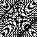
The first synthetic images we ought to manipulate are the Scilab-produced circle of certain radius and a Paint-produced image of the capital letter “A“. To start things off, we produced the synthetic image of the circle using the technique we used in previous activities. The image for “A” was produced in Paint by setting its properties to 128 pixels x 128 pixels and placing a white letter “A” in the middle of a black background. The synthetic images for this activity are all in 128 x 128 bitmap format. We took the FT of these figures and displayed their intensity values using the absolute value function, abs(). Since the output of FT has quadrants along the diagonals interchanged, we need to apply fftshift() to our resulting intensity values to rearrange the quadrants back to normal. The results are as follows.
Note: For this entire part of the activity and for each synthetic image, the leftmost image pertains to the original Scilab or Paint produced image. The next image is the FT of the synthetic image while the next image is the grayscale shifted version of the FT. The last image refers to the application of FT twice to the synthetic image. Also more often I would deal with the shifted FT of these images since these images are of interest for this activity.

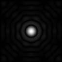


We can observe that the FT of these images definitely shows the interchanging of the quadrants along the diagonals. Upon shifting the obtained FT and converting the values to grayscale, we certainly can observe the real FT of these images. As for the FT of the circle, we can observe a known phenomena called Poisson spot as the pattern being shown. Poisson spot happens when a light is blocked by any circular aperture. This is consistent with the analytical FT of a circle. From this point, I can infer that if we consider our shapes as aperture, the FT of these shapes produced the interference pattern if a light strikes these apertures. Upon trying different radii for the circular image, I observed an interesting pattern in the results. The larger the radii, the smaller the observed spot is. This is true for interferometry where the smaller the aperture, the more visible the interference pattern that could be produced.
I cannot simply tell the same for the image of A since we never have an aperture of such shape but we can also use our intuition that based on its FT, we may have a case here about FT producing the interference patterns if the shapes are considered as apertures. The last images shows that the inverse FT is the same as the forward FT with the image inverted. This property can clearly be observe with the image of A.
To show that the FT of any function is complex, it is necessary for us to show the real and imaginary parts of the FT of the circle and image of A. The first 2 images are for the circle and the last 2 is for the image of A. The leftmost images for each are the real parts of the FT while the next images are the imaginary parts of the FT. From these images we can clearly confirm that the FT of any function is complex.
The next shape we simulated is the sinusoid along x more like a corrugated roof. The results are as follows.


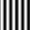
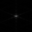
The most tricky image for this activity is this sinusoid. I believe a lot of people in class including me experienced a hard time obtaining an acceptable result for the FT of this image. We never considered the fact that the periodicity of this function ranges from -1 to 1. A bias was needed to lift the negative values of the function. Normalization was also necessary to dictate the range of the values as 0 to 1. I personally want to thank Dr. Soriano and Mario Onglao for shedding some needed light in this particular shape of interest. If we look closely at the FT of the sinusoid, we can find it at the top of the image. Shifting the obtained value, we can observe 3 dots. The analytical FT of a sine function with the form 
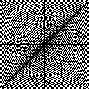
The next shape considered is the double slit. The process of doing the synthetic image in Scilab was fun because I thought of ways to make the slit as thin as possible yet I believe I made a blunder by putting too much distance between the slits.


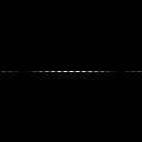

Again, the FFT lies on top of the entire black background. The third image shows the shifted FT of the double slit. We can observe a fringe pattern very common to the double slit. The fringe patterns are produced when a light strikes the double slit which causes interference among the waves. The hypothesis I created a while ago now more strongly suggests that the FT of these shapes produces patterns that in real situations happens when we consider a light striking the aperture with the shape of the considered figure. We can also observe that it seems like a Gaussian wave guides the pattern. Much like a beat, a larger sinusoid covers the fringe patterns as we can observe the difference in intensity between the patterns in the middle with those in the outer area of the shifted FT. I also want to thank Mario Onglao for pointing this concept to me while we were discussing the right result for this shape.
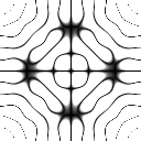
The next shape I would discuss is the square shape. The results are as follows.


If we were able to zoom in at the FT of the square shape, we might be able to see a cross shape pattern with the middle part of the pattern with the highest intensity. The change of intensity varies radially along the x and y axes. The same can be observed when we consider a cross shape aperture.
The last image considered for this part of the activity is for the 2D Gaussian bell curve. The results obtained are as follows.


Before I discuss the results for this synthetic shape, I would like to thank Dr. Soriano for pointing out my mistakes in the code for this simulation. I forgot to include a σ in the Gaussian equation. Also the mesh in Scilab was helpful for checking the correctness of the Gaussian bell produced. The FT of this shape is also a Gaussian curve of larger area. When we apply the FT inversely, we also obtained a Gaussian function of larger area. This is consistent with the analytical FT of the 2D Gaussian bell where we really obtain another Gaussian with a larger area.
Simulation of an imaging device
This part of the activity projects the properties of the concept of convolution. In particular, the linear operation can be represented in linear transformations such as Laplace or Fourier. We can observe convolution by simply multiplying the FTs of the functions of interest.
Using Paint, a 128×128 bitmap image of the word “VIP” was created. A circular image of a certain radius was also made using Scilab. We load these images in Scilab and obtained their FTs. Since the circle is already in the Fourier plane, we only obtained the shifted FT of the circle. The circle serves as the aperture of the circular lens. I believe this is the part where I would be able to confirm my hypothesis a while ago that FT serves as a lens for the patterns created for an aperture of certain shapes.
We get the product of their FTs and to observe their convolution we get the inverse FT of the product. We tried this for different radii of the circle. These are the results by using circular apertures of radius 0.3 to 0.9 with intervals of 0.1. The order of results is increasing radius from left to right, top to bottom.


The first image is the original “VIP” image produced in Paint. As we can observe with the results, with increasing radius of the circle, the clearer the image. As expected, this should be the result since increasing the size of the aperture should allow a higher of intensity of light to pass through. The image also has the properties of both the circle and the VIP image. The results are also consistent with the relationship between the inverse and forward FFT.
Template Matching using Correlation
Correlation is similar to convolution by having a correlation theorem which also holds for linear transformations. It has basically the same form as the convolution but a term is conjugated. The process is the same and the change we make is to obtain the complex conjugate of the FT of the image of interest. The image of interest is shown as the first image below.
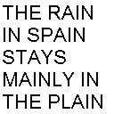
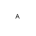 The image of A has the same font and font size as the phrase shown in the image of interest. Correlation measures the degree of similarity between two functions. The more identical the functions at certain coordinates, the higher their correlation value at that coordinate is. The concept of correlation is mostly used in template matching or pattern recognition. The aim of this part of the activity is to numerically obtain the correlation of these two images. The result of their correlation is shown below.
We can observe that the parts of the image with the highest intensity are those areas where a letter “A” is located. Definitely the correlation of the images are obtained using the given process. We can definitely use Fourier transform and the correlation theorem for template matching and pattern recognition given that we have the image of the desired pattern or template.
Edge detection using the Convolution Integral
The last part of the activity aims to combine the concept of convolution and the correlation theorem to perform edge detection. We use the concept of template matching in correlation to find edge patterns in an image. The image of interest is the VIP image used for the 2nd part of the activity.

A 3×3 matrix pattern of an edge is made using Scilab. The values inside the matrix has a total sum of zero. This pattern was placed in the middle of a 128×128 black background image. Different patterns were produced: horizontal, vertical, diagonal and a spot pattern. The images containing the patterns are convolved to the VIP image. The results are as follows:


The first image is produced by the image containing the horizontal pattern. We can observe that correlation is achieved since we can see the emphasis or the higher intensity of values in the horizontal areas of the VIP image. The highlight of the image lies on the horizontal areas. We can also observe this in the 2nd image, produced by the vertical pattern containing image. The 3rd resulting image produced by the diagonal pattern containing image also highlights the diagonal areas of the VIP image. The spot pattern image produced the 4th image giving us the edge of the VIP image. I found it cool that the spot pattern gave us the entire edge of the VIP image. It means that we can get the edge of any image by convolving it with an black image with a spot pattern centered in it.
The activity provided a lot of fun and anxiety as well. I thought some of my results are blotched or mistakes but I found some relief by asking some of my classmates. I want to thank Ron Aves for providing me with some tricks for Scilab to read the right kind of data type for my images. Hats off to Ralph Aguinaldo who confirmed my results in the template matching part. All along I thought I made a mistake but then I realize that the intensities should really be high at different parts of “A” in the image. Also I made a mistake of not placing the 3×3 patterns in the middle of a 128×128 black image which made me wonder why my code won’t work. And of course I want to thank Dr. Soriano for providing inspiring messages and short motivational speeches to boost our morale.
Overall, I give myself a 10 for the effort I gave for this activity. I think I allotted enough time to accomplish this activity. I don’t deserve extra points since I stuck to the required tasks and did not try anything beyond the required tasks. But overall I am happy with the new lessons and techniques I learned through these activities.

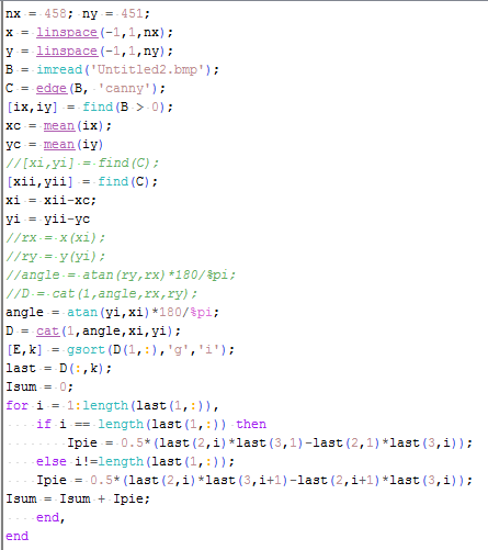
![A=\frac{1}{2}\sum\limits_{i=1}^{N_b} [x_{i}y_{i+1}-y_{i}x_{i+1}]](https://s0.wp.com/latex.php?latex=A%3D%5Cfrac%7B1%7D%7B2%7D%5Csum%5Climits_%7Bi%3D1%7D%5E%7BN_b%7D+%5Bx_%7Bi%7Dy_%7Bi%2B1%7D-y_%7Bi%7Dx_%7Bi%2B1%7D%5D&bg=ffffff&fg=333333&s=0&c=20201002)


 or 0.4644
  . Knowing the length of the ID, I drew a straight line to the length of the image. I set the scale by using Analyze > Set Scale… placing the known distance. The scale is given by 1169.14 pixels/m. By placing a polygon (rectangle) in the ID, we measured the area by using Analyze > Measure. The computed area for the ID is 0.455
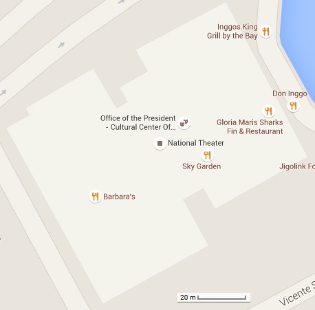

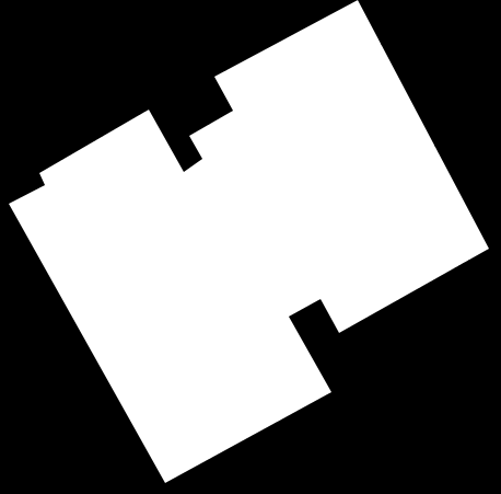
 . Using the scale in ImageJ, I converted the pixel area in to real area. The computed Scilab area is 8207.7015 sq. meters. Using ImageJ, I was able to compute an area of 8191.388 sq. meters. I obtained a deviation of 0.2%. I could say that the Scilab code was effective in computing the area of the National Theater of the Philippines.