And at last we arrive at this moment. This is the time to blog about the last activity of Applied Physics 186. This is the last activity of the sem and hopefully my last required blog for my bachelor’s degree. 🙂 This subject gave me some new skills that I know I would be able to effectively use for other purposes at some time. And one of them is this activity, basic video processing.

A video could be viewed as a set of images that are in sequence with one another shown in very rapid succession. Because of this concept, we would be able to study in detail the motion of an object or how something spreads. There are many practical applications of video processing such as the study of the growth of a bacteria, the motion of an athlete in sports and the motion of a falling object.
Each digital video has a frame rate or fps which indicates the number of frames or images that the camera we used can capture in a second. This means that for every pair of succeeding image has a time interval of the inverse of the frame rate. By knowing these concepts, we can study the time dependent parameters using images from videos such as a motion of an object.
For this activity, we investigate the free fall of an umbrella. We go back to the concept of kinematics to observe the motion of the object. Without air resistance, the object has an acceleration equal to g, or 9.8 m/

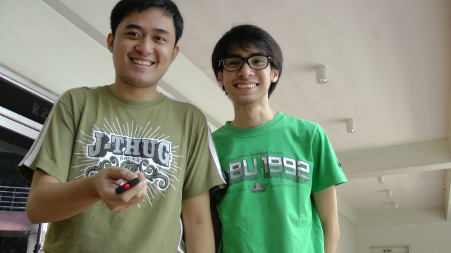
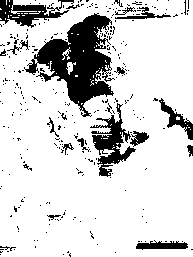
In this activity, I paired up with Martin Bartolome to investigate the free fall of an umbrella. First and foremost, I would like to thank our hero, Mario Onglao for lending us his blue umbrella without hesitation. Without your kindness, this activity would not have been possible for us. And as proof that we performed this experiment, first let us take a selfie!
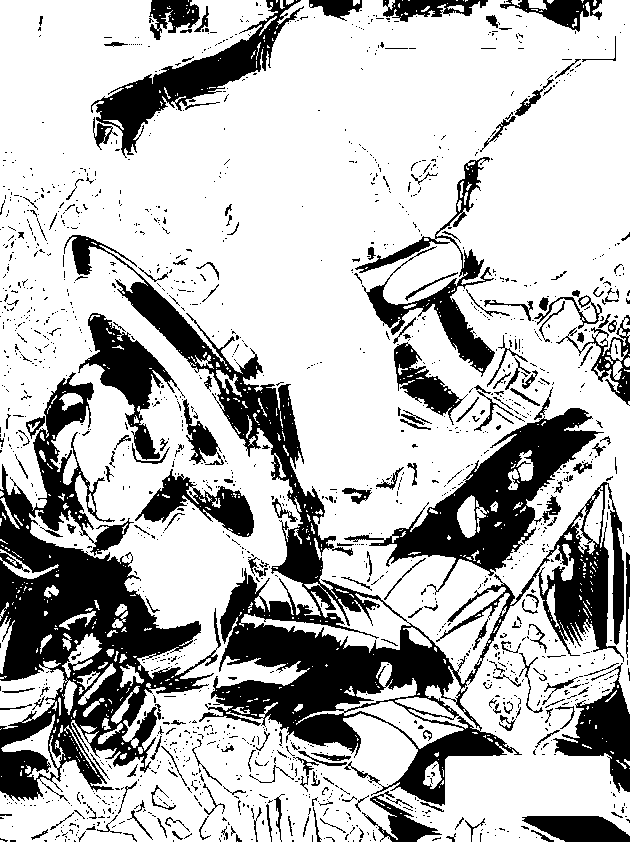
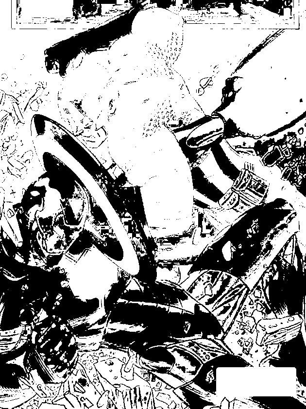
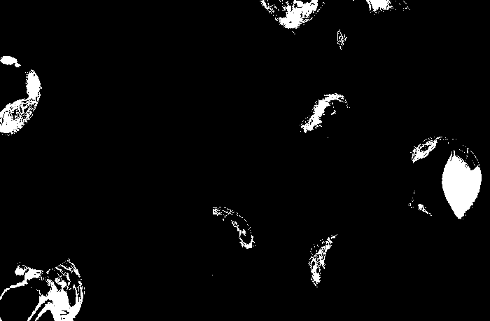
We took advantage of the height of the very beautiful NIP building to perform the experiment. We drop the umbrella from the fourth floor of NIP and Barts received the umbrella at the ground floor. With the help of Dr. Soriano (maam thank you!), we were able to capture the experiment using her Olympus DSLR camera. We present a GIF version of the video.
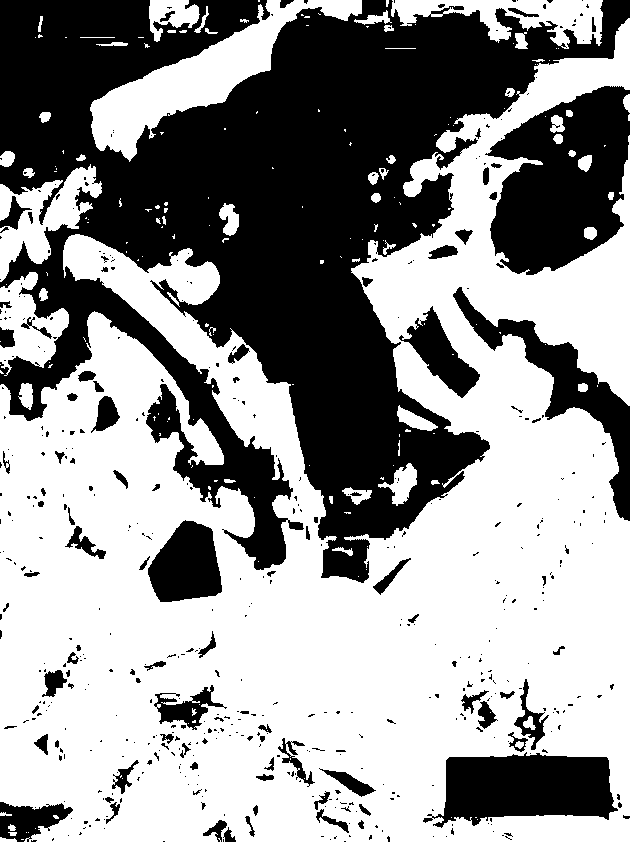
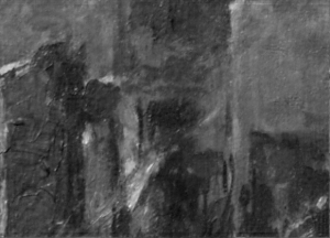
Figure 1: GIF version of a portion of the original video clip which shows the free falling of a blue umbrella
The GIF image is from a 4 second clip from the original video captured. It features the exact time I released the umbrella until it reaches the hands of Barts. It is obviously slower than the original pace of the video for its purpose if for us to at least observe the motion of the umbrella as it reaches its terminal velocity. And by observation we could observe this phenomenon and we wish to prove it using the video processing technique. But first I want to note that the camera used has a frame rate of 59 fps. Since this would require me to have a large number of images to be processed, I chose to reduce the frame rate to 15 fps for my analysis. I think that the chosen frame rate would be enough for this purpose.
To perform video processing, we must first obtain the images by any software that could help. According to the manual given to us, some suggested softwares are STOIK Video Converter for video format conversion and VirtualDub for extracting images from the video. But there was a problem with the format of the video we have. It is in MTS format and the STOIK Video Converter cannot convert this so we cannot use these softwares. Good thing I ask Gio Jubilo for some help and he pointed out about some video to jpg converter. Upon searching, I found the free DVDVideoSoft software. It contains a Video to JPG converter mode. This is the software I used to extract the images from the video. I used the parameter 15 fps to extract the images from the video.
We note again that the time interval between succeeding images I obtained is the inverse of the frame rate. So the time interval is equal to 1/15 or 0.0667 seconds which should be enough for a 4 second clip for video processing. Of course with a choice of a larger frame rate, we could be assured of a higher accuracy of analysis but also a higher need of processing power. The choice of frame rate for image extraction should depend on the purpose of the user.
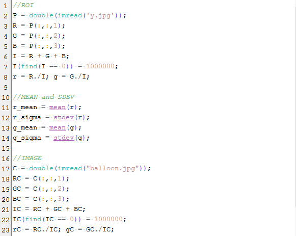
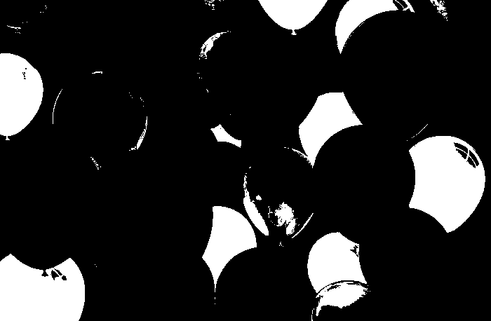
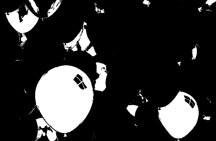
From these images we would be able to determine the velocity of the umbrella during its free fall. For the sequence of image, we could locate the centroid of the umbrella and know its distance from the initial position. We would be able to do this by image segmentation as we previously learned from Activity 7. Since we have the skills for this purpose, we can immediately go through the process. There are two kinds of image segmentation and from the activity, we observed that the non-parametric segmentation is the more flexible and efficient method. Even though it requires a lot of processing time, the results are unmatched. For this activity, I applied the non-parametric segmentation to the 61 images obtained and used the patch shown below as our region of interest (ROI).

patch
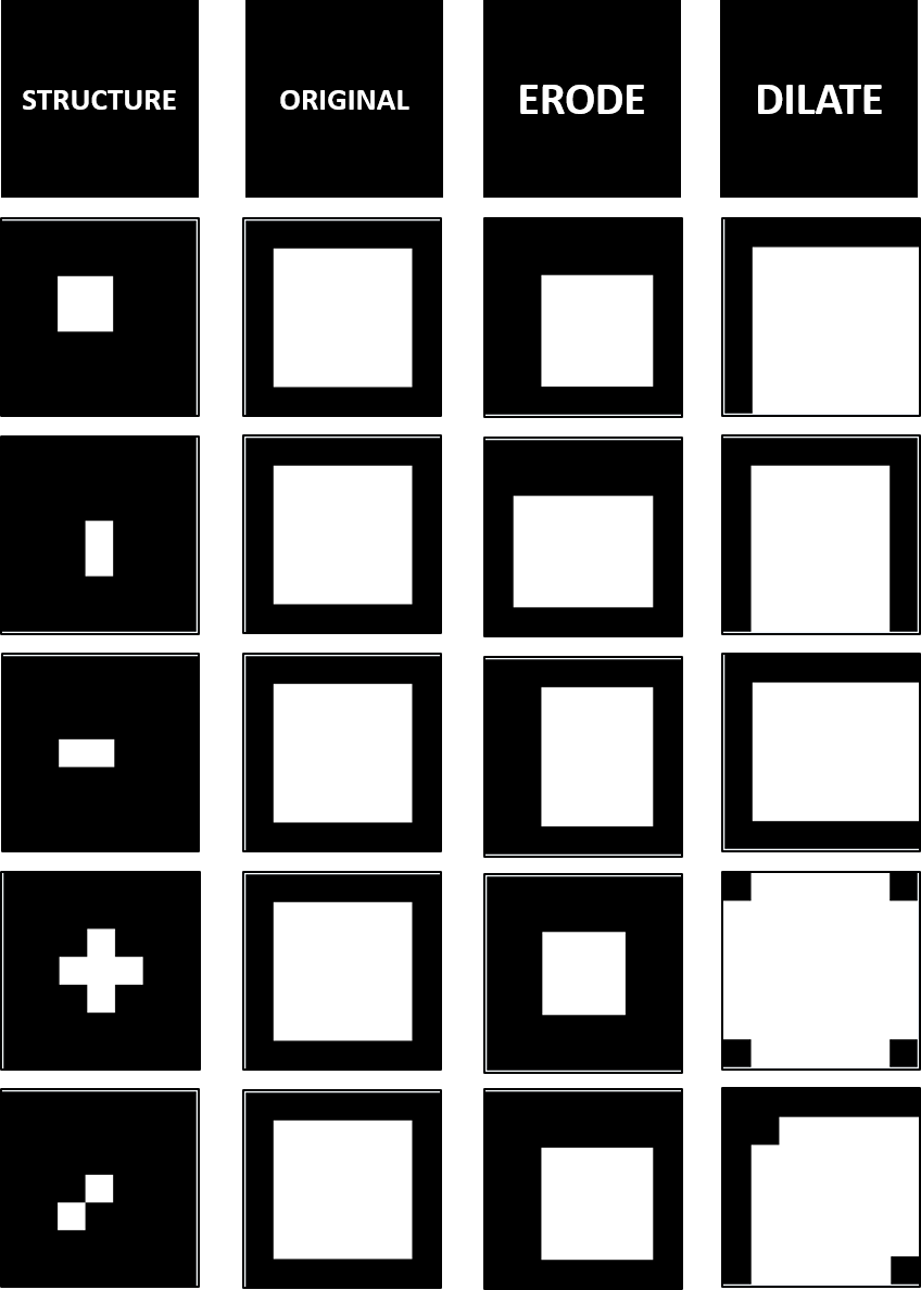
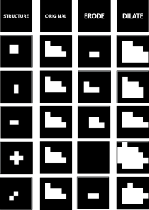
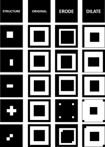
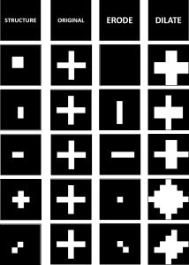
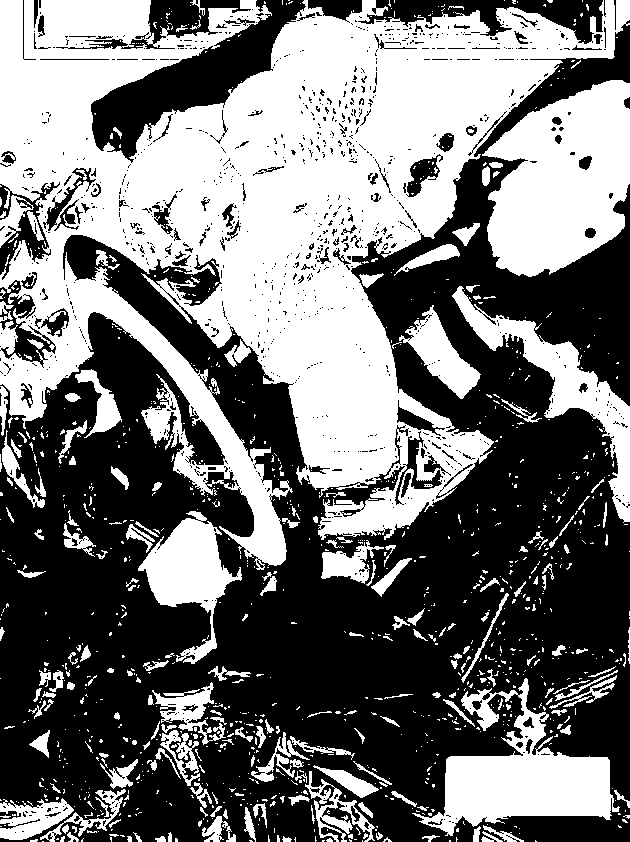
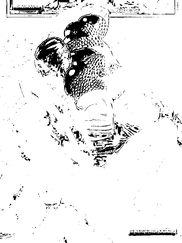
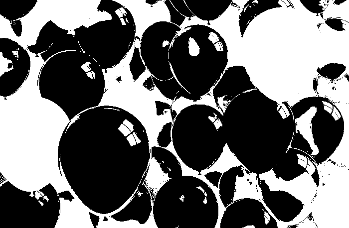
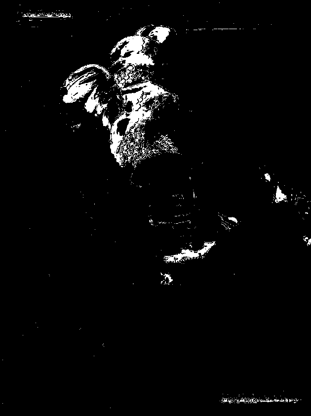
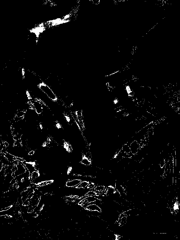
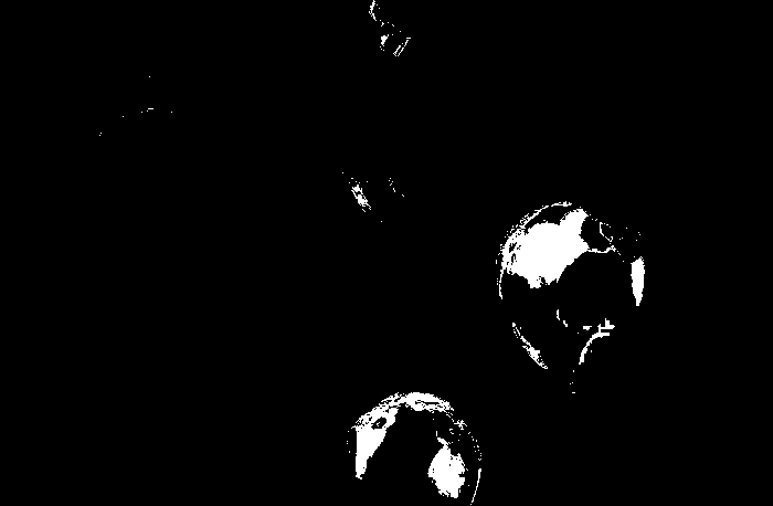
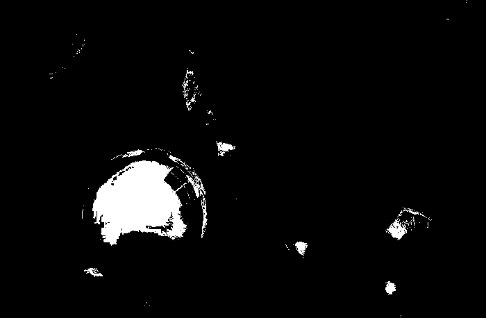
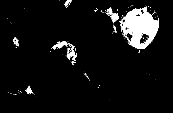
The patch is a part of the umbrella. Good thing that the color of the umbrella stands out from the background therefore we were able to segment the umbrella from the surrounding. After segmenting, we observe that there are still stray intensities away from the location of the umbrella. This problem would affect our search for the location of the centroid of the umbrella for each time step. Therefore learning about morphological operations in Activity 8, we know that we could remove these stray values and retain the shape of the umbrella. We use the Open operator and a circular structuring element of radius 7 pixels to clean the stray intensities and retain the shape of the umbrella. The operator first erodes the stray values then dilates or maintain the shape of the umbrella. After doing all these image segmentation and morphological operations, the finish product is shown in GIF format below.

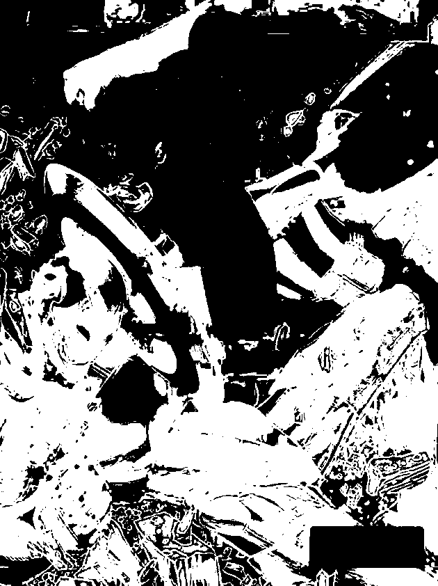
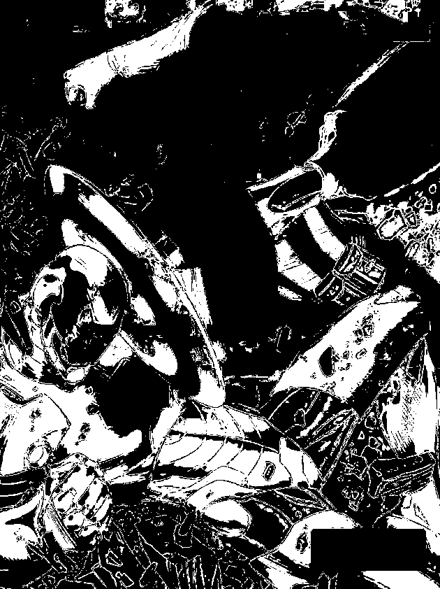
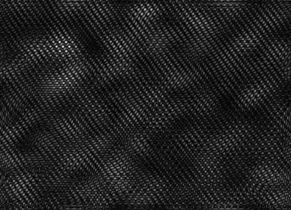
Figure 2: GIF version of the segmented images from the video. The morphological operator, Open, was also used.
The patch I used to segment the umbrella is from an image where it is still on top of the 4th floor. From the original clip of the video, we can observe that at the start of the free fall, the umbrella is illuminated by the sun. The patch is from this portion of the video which can also explain the diminishing shape of the umbrella. The morphological operator, Open, might also be a cause for the diminishing shape. There was also a part of the motion where the umbrella partly tilted in the z-axis therefore the shape diminished at that point. The centroid was calculated by taking the mean value of the coordinates of the white pixels of the segmented shape of the umbrella.
The distance is calculated for each centroid of every image from the initial position. Knowing the time step for each pair of succeeding image, we plot the distance vs time plot. But before I forget, first things first. We took the distance of the centroid in pixel units. We convert this into a real physical unit. We were able to measure the distance between the floors of the second and third floors of the building which is 84 inches. By using this measurement, we learned that the conversion factor is 0.168 inches / pixel. The plot is shown below.
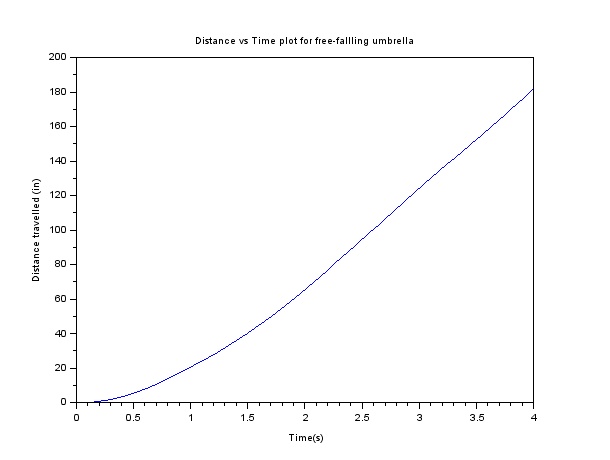
Figure 3: Distance vs Time plot for the free fall motion
And voila! The object seems to pick up its velocity in the first moments then maintain a steady velocity in the later parts of its free fall. This velocity is our terminal velocity where the drag force is already equal to the force of gravity on the object. We simply take the slope of the linear plot to obtain this value. I tried to plot the linear regression using Scilab but then I do not know how to place the equation of the line in the plot’s legend. I used Excel instead to plot the linear regression of the plot. Fortunately, the equation of the line I obtained in Scilab is the same with the Excel plot I obtained. This is the linear regression of the plot of the distance vs time of the free fall of the umbrella.
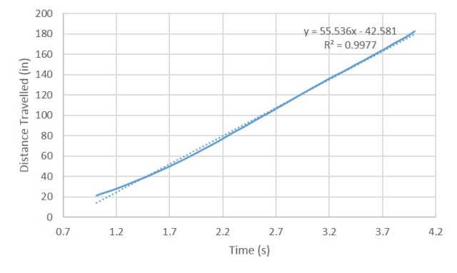
Figure 4: Linear Regression of the linear plot
You can observe that I cut the plot and started at about 1 second since the umbrella was still picking up its velocity on earlier times as shown by the curve of the motion plot. We obtain a 55.536 slope which means that the terminal velocity is 55.536 inches/second or about 1.41 m/s which is realistic. We can also observe this in the original video clip we have.
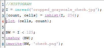
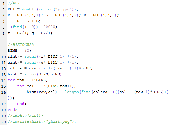
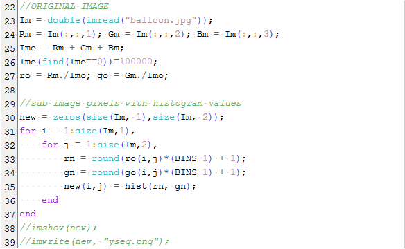
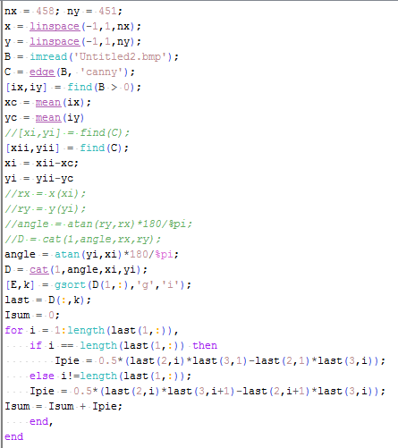
By this experiment, we prove that we can use video processing to investigate some physics concepts and obtain good data. I am very thankful for this activity because I was able to use some other skills I learned from previous activities which was really fun. I hope that I can still use these skills in the near future. And ooops, before I end this activity, these are snapshots of my Scilab code I used for segmenting, application of the morphological operator and plotting for this activity.


For this activity, I would like to give myself a 10/10 since I was able to present the concepts and results properly. I was also able to perform the skills and technique well. I want to also give myself an extra 2 points since I believe that I presented a great quality of work. By this self-evaluation, I end my Applied Physics 186 blog series. I hope I can still post some time on this blog and share some more things I would learn in the future. Thank you Maam Jing for these new skills and fun you showed us through these challenging activities. We will cherish these activities which I know are out of the box activities. 😀
And since this is the last activity blog, please bear with me with these emotions.


And because I am really happy, please give me some.

 B = { z |
  ∩ A ≠∅ }
 ⊆ A }
⊆ A }
 =
= 


 ,
,  ,
, 
 . We can take note that
  . We further simplify the coordinate system by setting the dependence of the blue channel with red and green channels,
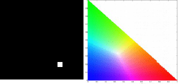
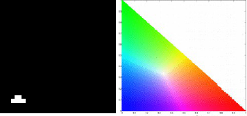
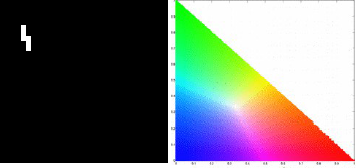
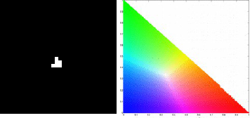
  . We then can represent chromaticity with just two coordinates, r and g. The variable I would contain brightness information. The NCC can be seen as such.
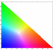


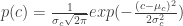
 and
and  are the mean and standard deviation from the pixel samples. To tag a pixel as belonging to the ROI, we would consider the joint probability,
  .
.


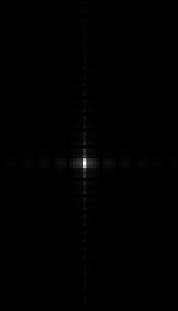


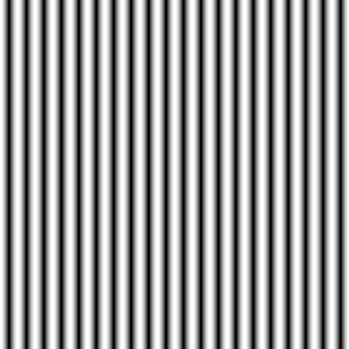

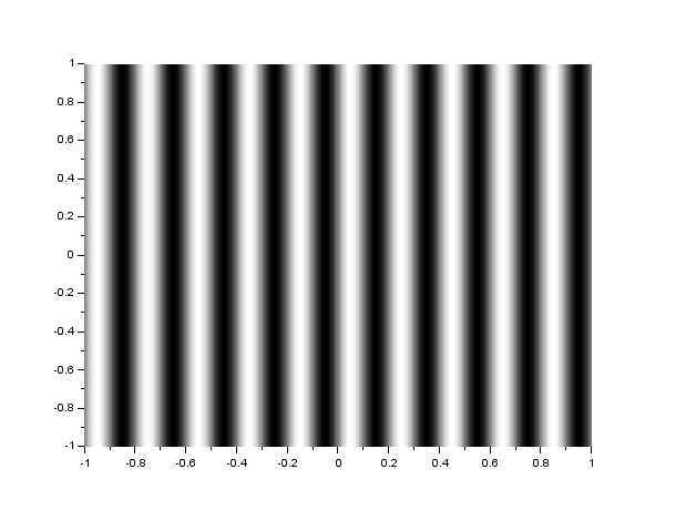
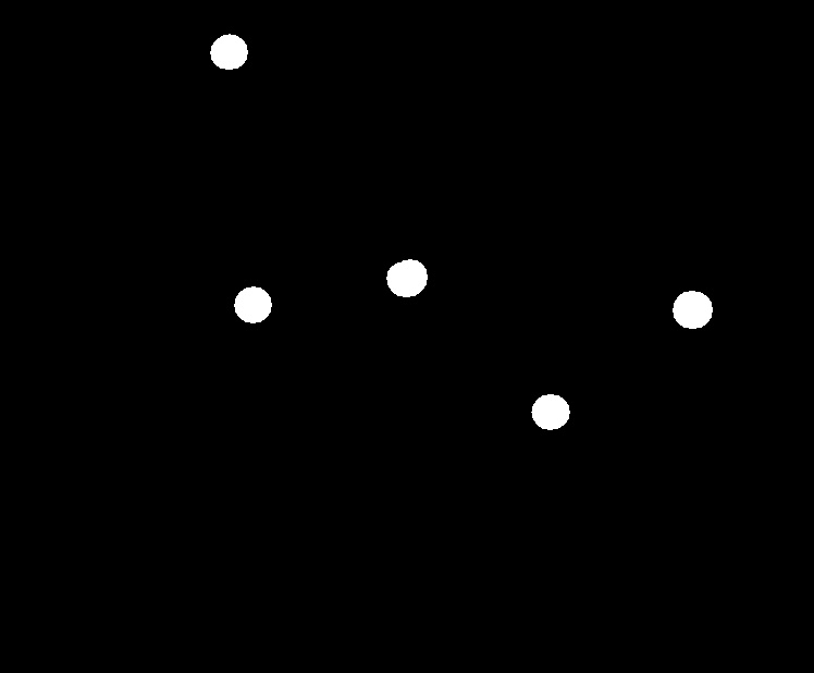
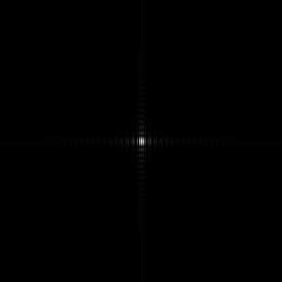
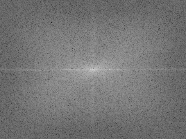
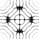
 where f is the frequency. Its FT was obtained and the FT modulus was displayed. With a frequency of 4, the sinusoid and its FT is shown below.


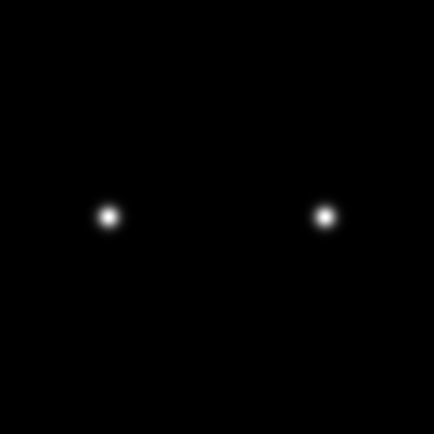
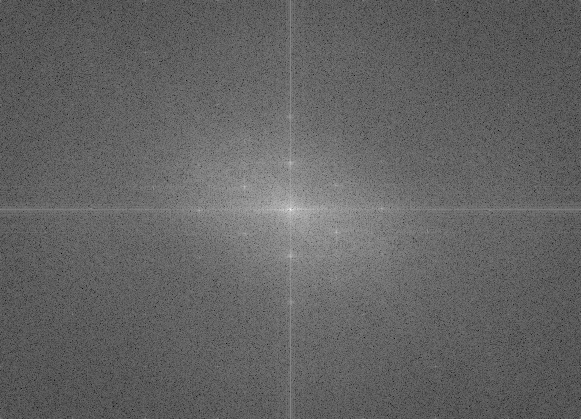
 , we obtained the following results. We can observe the spacing of two dots increases as the frequency of the original sinusoid is increased. We can also observe another set of 2 dots in the middle which can be attributed to the very low frequency added. So for an interferogram setup where a non-constant bias is added, we still can determine the frequency of the interferogram by simulation and the use of Fourier transform.


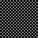
 , the new sinusoid form is in the form
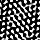
  . The resulting images and their FTs for different frequencies is shown below.


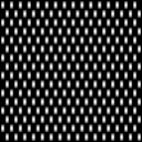
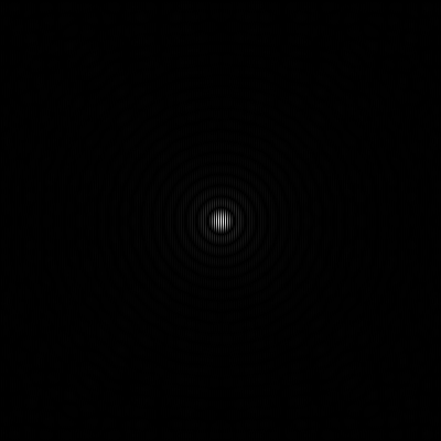
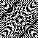
 in different axes and their resulting FTs are shown below.
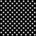


 of varying


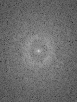


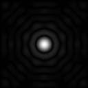


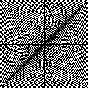


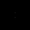
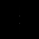
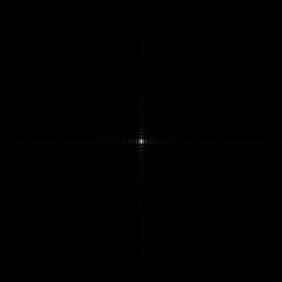
 includes the Dirac delta function with peaks at k and -k. The obtained FT clearly shows the equally spaced dots from the center pertaining to the frequency of the sinusoid, k. The last image also follows the relationship between the inverse and forward FFT.


![A=\frac{1}{2}\sum\limits_{i=1}^{N_b} [x_{i}y_{i+1}-y_{i}x_{i+1}]](https://s0.wp.com/latex.php?latex=A%3D%5Cfrac%7B1%7D%7B2%7D%5Csum%5Climits_%7Bi%3D1%7D%5E%7BN_b%7D+%5Bx_%7Bi%7Dy_%7Bi%2B1%7D-y_%7Bi%7Dx_%7Bi%2B1%7D%5D&bg=ffffff&fg=333333&s=0&c=20201002)


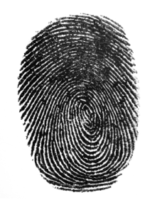
 or 0.4644
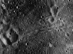
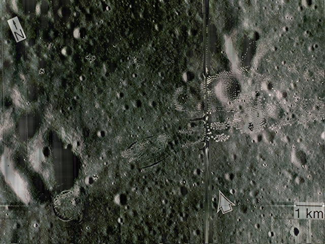
  . Knowing the length of the ID, I drew a straight line to the length of the image. I set the scale by using Analyze > Set Scale… placing the known distance. The scale is given by 1169.14 pixels/m. By placing a polygon (rectangle) in the ID, we measured the area by using Analyze > Measure. The computed area for the ID is 0.455
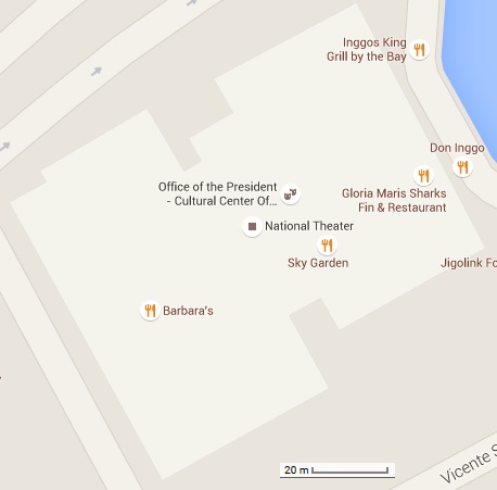


 . Using the scale in ImageJ, I converted the pixel area in to real area. The computed Scilab area is 8207.7015 sq. meters. Using ImageJ, I was able to compute an area of 8191.388 sq. meters. I obtained a deviation of 0.2%. I could say that the Scilab code was effective in computing the area of the National Theater of the Philippines.