Our goal for this activity is to reconstruct a hand-drawn graph to a digital graph using the concept of ratio and proportion in pixel and physical values. From pixel values we must acquire a relationship that would relate the pixel values to the actual physical variables in the graph.
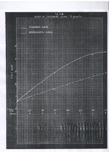
The truth is the hardest work I encountered in this activity is finding a hand-drawn graph. We tried going to NIP library to find a hand-written graph. We found some old thesis and journals but we were not satisfied with the graphs we saw. We thought that we need a really obvious hand written graph. Actually, the process of finding the graph was really frustrating. We approach the last day of the week and we haven’t found any graph yet. Good thing is that Robert Tacbad and Jaime Olivares were with me when I visited the CS library to find some really old thesis. It was full of very old journals and published works. We came through a shelf that were published from 1950-1960. Jackpot! Then we came through another problem, the sensitivity of rules about these works restricted us from simply photocopying or scanning the graphs we found. We thank the CS staff members that were very understanding. You da real MVPs. At last they understood that we would not in any way plagiarize or use these graphs for any to-be-published work. We promised we will cite our references. The graph I obtained came from a thesis by a graduate student named Nieves Portugal-Dayrit entitled “The Microbiological Assay of Amino Acids in some Philippine Legumes” published in February 15 1956. My grandpa was just 12 years old back then. Wow!

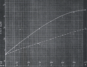
The process of reconstructing the graph started by producing a digital image of the graph. We had a photocopy of the graph from CS and finally we scanned it in our laboratory to acquire our image. I cut the obtained image to focus on the graph itself. Using GIMP 2.8, I acquired pixel locations of the x and y axes of the graph. I must say that I am very lucky since the film used to plot the graph has some grids that made it easy for me to acquire pixel locations. Using these data, I acquired an equation that relates the physical variables to the pixel locations. For the x axis variables, I obtained an equation: x_phy = 0.0062x_pix – 1.2081 while for the y axis variables: y_phy = 0.0025y_pix – 0.4993 where subscripts phy pertains to physical variables and pix to pixel variables.

I turned my attention to the graph itself. I acquired the pixel locations first of notable locations of the graph. I tried to graph the obtained data and observed that the first graph was still rough. I collected more pixel locations in the graph summing up 22 points in the graph. I plotted the obtained data and observed that the graph somehow resembles the original graph. The first graph I obtained has axes in pixels.
![]()
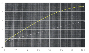
Using the equations for the relationship of the physical variables and pixel locations, I converted the axes into physical variables. The next step is to confirm the similarities of the original and the digitally reconstructed graph. Using Microsoft Excel, I overlaid the image of the original hand written graph to my digital graph. By placing offsets to align the axes of the image and the graph, I confirmed that I obtained the same graph as the original hand-written graph. From this confirmation, I give myself a 10 for this activity. I also want to note that the axes of the original image have the same axes values with the Excel graph. The values were obtained from the equation.
![]()

Reference:
N. Portugal-Dayrit, “The microbiological assay of amino acids in some Philippine legumes,” College of Science, University of the Philippines Diliman, 1956.