Activity 2 – Digital Scanning

Our goal for this activity is to reconstruct a hand-drawn graph to a digital graph using the concept of ratio and proportion in pixel and physical values. From pixel values we must acquire a relationship that would relate the pixel values to the actual physical variables in the graph.

The truth is the hardest work I encountered in this activity is finding a hand-drawn graph. We tried going to NIP library to find a hand-written graph. We found some old thesis and journals but we were not satisfied with the graphs we saw. We thought that we need a really obvious hand written graph. Actually, the process of finding the graph was really frustrating. We approach the last day of the week and we haven’t found any graph yet. Good thing is that Robert Tacbad and Jaime Olivares were with me when I visited the CS library to find some really old thesis. It was full of very old journals and published works. We came through a shelf that were published from 1950-1960. Jackpot! Then we came through another problem, the sensitivity of rules about these works restricted us from simply photocopying or scanning the graphs we found. We thank the CS staff members that were very understanding. You da real MVPs. At last they understood that we would not in any way plagiarize or use these graphs for any to-be-published work. We promised we will cite our references. The graph I obtained came from a thesis by a graduate student named Nieves Portugal-Dayrit entitled “The Microbiological Assay of Amino Acids in some Philippine Legumes” published in February 15 1956. My grandpa was just 12 years old back then. Wow!

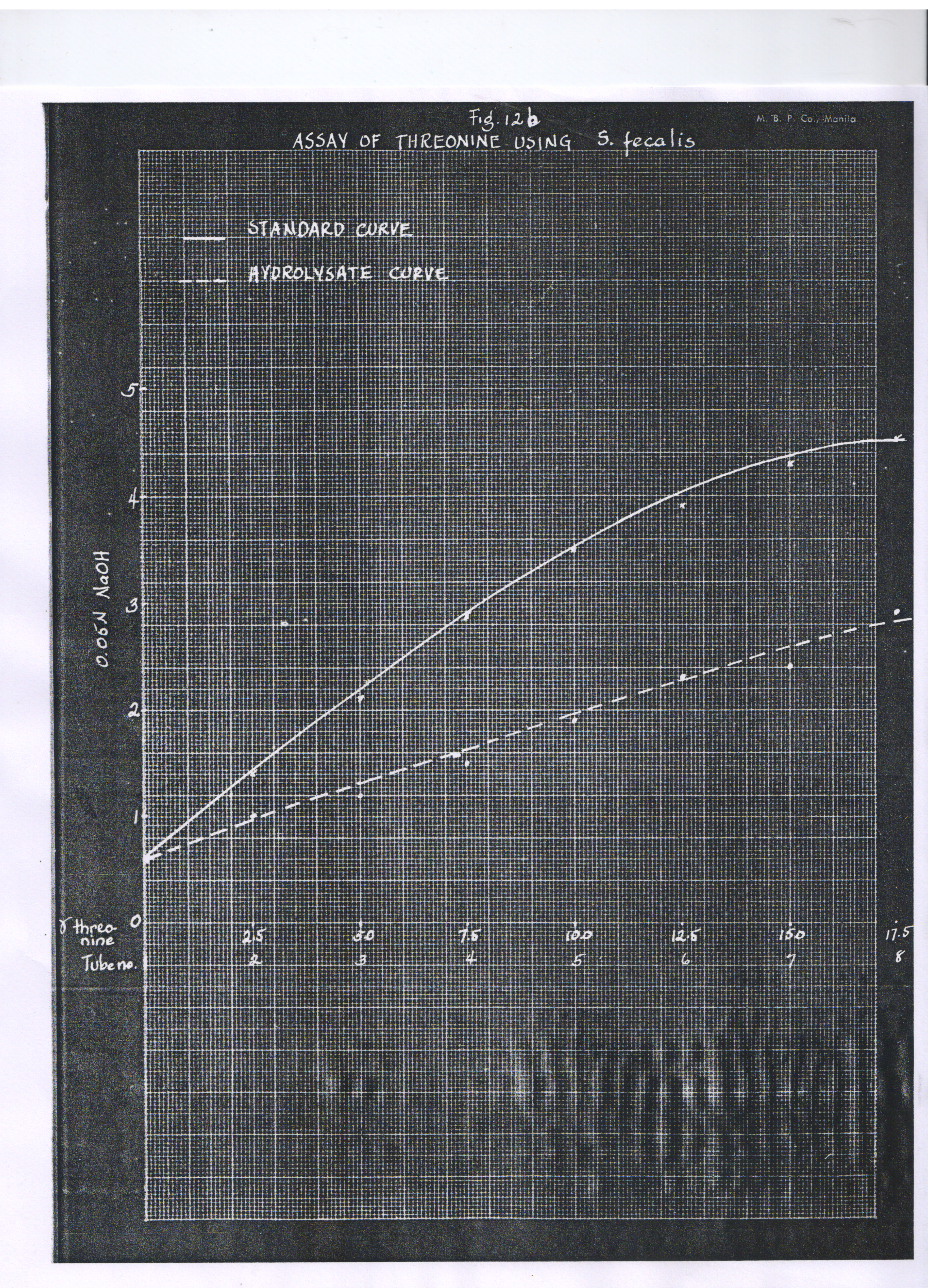
The process of reconstructing the graph started by producing a digital image of the graph. We had a photocopy of the graph from CS and finally we scanned it in our laboratory to acquire our image. I cut the obtained image to focus on the graph itself. Using GIMP 2.8, I acquired pixel locations of the x and y axes of the graph. I must say that I am very lucky since the film used to plot the graph has some grids that made it easy for me to acquire pixel locations. Using these data, I acquired an equation that relates the physical variables to the pixel locations. For the x axis variables, I obtained an equation: x_phy = 0.0062x_pix – 1.2081 while for the y axis variables: y_phy = 0.0025y_pix – 0.4993 where subscripts phy pertains to physical variables and pix to pixel variables.

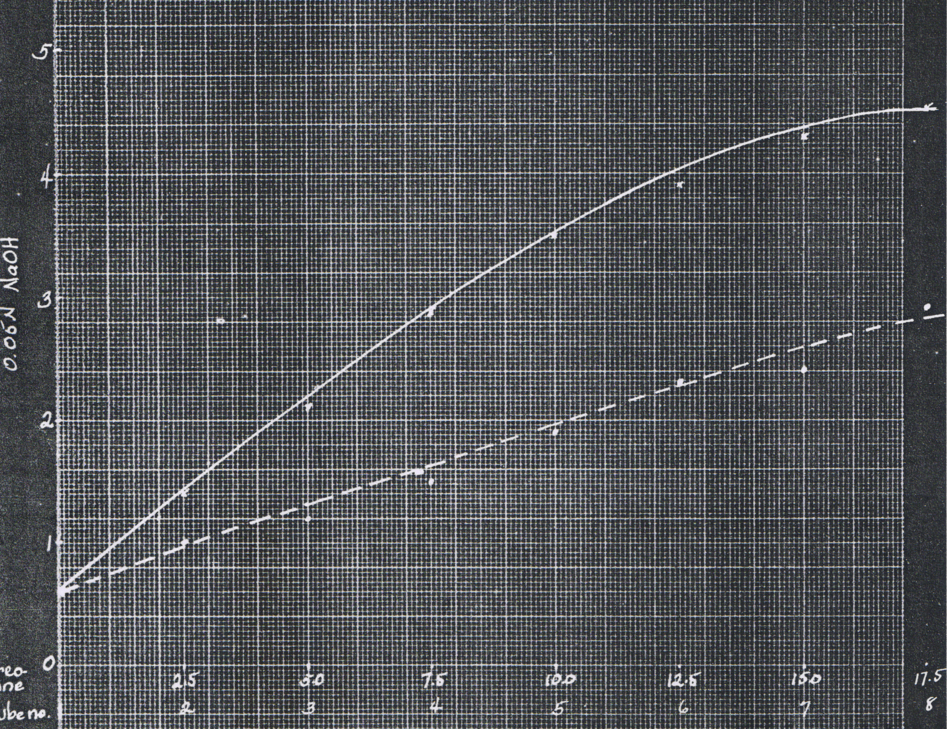
I turned my attention to the graph itself. I acquired the pixel locations first of notable locations of the graph. I tried to graph the obtained data and observed that the first graph was still rough. I collected more pixel locations in the graph summing up 22 points in the graph. I plotted the obtained data and observed that the graph somehow resembles the original graph. The first graph I obtained has axes in pixels.

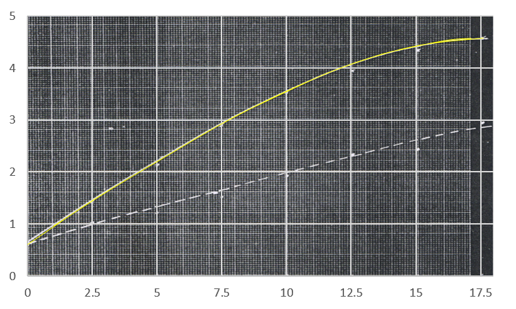
Using the equations for the relationship of the physical variables and pixel locations, I converted the axes into physical variables. The next step is to confirm the similarities of the original and the digitally reconstructed graph. Using Microsoft Excel, I overlaid the image of the original hand written graph to my digital graph. By placing offsets to align the axes of the image and the graph, I confirmed that I obtained the same graph as the original hand-written graph. From this confirmation, I give myself a 10 for this activity. I also want to note that the axes of the original image have the same axes values with the Excel graph. The values were obtained from the equation.

Reference:
N. Portugal-Dayrit, “The microbiological assay of amino acids in some Philippine legumes,” College of Science, University of the Philippines Diliman, 1956.

Activity 3: Scilab Basics

Activity 3 tackles with us playing with Scilab. Honestly, I have little knowledge of the software since I used this software for an activity last semester for our Applied Physics 185 class also with Dr. Soriano. But what I did last year was different since it involves Fourier transform and the synthesis of sounds. What we aim for this activity is to create synthetic images with the use of matrices and basic arithmetic. We were given an example of a Scilab code to create a circular aperture or a pinhole. The image produced shows a black background and the white circular portion pertains to the aperture. Basically, we aim to produce different images with this style.

The task given to us was to produce 7 specific images. It was a fun activity since it relies on our imagination and wit on how to construct these images. At first I don’t have an idea of how to construct these images since I still worry about the basics of programming in Scilab. But I was grateful for the example given by Dr. Soriano because it made sense on how to construct these figures. And I want to thank all my classmates since we brainstormed our way into the light, that is, the basic things we need to know in producing a program to construct these figures.

The first figure I was able to construct is the ellipse. It was the easiest to figure out since we are already given the code for our circular aperture. I just reduce one variable to a fraction for our circular aperture to be an ellipse. It follows the equation for an ellipse knowing that a circle is a special case of the ellipse. I tried to produce a diagonal ellipse but I failed to do so since my code does not work due to an issue of the use of the element-by-element operator “.” when doing the operations. The centered square aperture and the cross were somewhat connected. I constructed the cross figure by thinking of strips. I imagined two strips in the center parallel to x and y axes overlapping to form a cross. I also tried to make a smaller version of this cross and came up with a new figure. This figure symbolizes more of the cross we commonly know. With this idea, I immediately thought of how to construct the square. I first built a strip parallel to the x-axis then cut the strip in its end to construct the square. I made sure that sides of the square are equal.

Using the example of the circle, I thought of just placing a black smaller circular aperture in the constructed circle. This formed the annulus and voila I completed another figure. At this point, I am starting to enjoy the process of learning the basics of Scilab since I am getting the feel of it. I stopped a bit when I tried to figure out how to construct the sinusoid along the x-direction. The corrugated roof seems a little complicated for me. I would like to thank Martin Bartolome and Jesli Santiago for giving us some tips for the 2 of the last 3 figures. Since it was obvious that we need a sinusoid for the corrugated roof, we just simply plotted a sinusoid knowing that it is periodic in nature. I was surprised that it was that simple. I was happy and worried at the same time since I think I am overthinking the process of constructing these figures. From the sinusoid, we can easily build the grating along the x-direction. By adding a grid of zeroes, for every certain value (0.8 for my figure) of the sinusoid, we replace the value of that sinusoid coordinate in our zero grid by 1. From this we produced the grating along the x-direction.

And at last I am about to construct the last required figure. Then it hit me, it is not simple. How do I make a circular aperture with graded Gaussian transparency? Jaime and I tried to find sources of how to do this. We searched the internet and tried the steps shown in our sources but to no avail. Upon searching for a Gaussian entry in the help window of Scilab we encountered the equation that describes the Gaussian distribution. I thank Jaime for pointing out that we can use the equation of the Gaussian transparency to form a “ripple-like” figure then we replace the values to 0 while retaining a circular aperture in the middle by applying the concept of the example given to us. In short, we first constructed a ripple effect in the grid then cover everything except for a circular aperture in the middle. I’m done! It was fulfilling to construct all these figures. Thank you maam for bringing fun to learning. It was refreshing in some way with all the stress of the past semesters at least I can say that I had more fun in this one.

I tried to play with our codes and I constructed different figures. From my code for the square aperture, I constructed a star like figure. I also tried to construct some strips. I tried some other figures but I failed to do so. I believe I deserve a 10 for this activity because I successfully constructed all the required figures. I think I also deserved an extra point since I tried to play with the figures. I had fun with this activity so I believe I deserve these self-given points.