Morphological operations are used in image processing to process or extract information from a binary image. Usually these binary images are aggregates of 1’s forming a particular shape. These morphological operations affects the shape of the image in any way. The shape might be expanded, thinned or closing of internal holes and disconnected blobs can be joined. For numerical calculation of this operation, we represent our black background with 0’s and our shape with series of 1’s.
The concept behind the morphological operations is the Set Theory. The concepts of being an element of a set (∉), subset (⊂), union (∪), intersection (∩), empty set (Ø), complement (C), difference (A-B), reflection and translation comprises the basic what to know about morphological operations. Combining all these concepts, we simplify and discuss just two of the morphological operations: Erosion and Dilation.
Dilation is defined as,
A 

B is defined as the structuring element. All z’s which are translations of a reflected B when intersected with A is not an empty set. Dilation aims to expand or elongate A in the shape of B. An example is given below.

Erosion is defined as,
A ⊖ B = {z| 
The erosion of A by the structuring element B is the set of all points z such that B translated by z is contained in A. Erosion aims to reduce the image A by the shape B. An example is shown below.

Erosion and dilation are duals of each other thus the relationship follows,
(A ⊖ 

Exercises
To observe erosion and dilation, we did an exercise to predict and observe the erosion and dilation of 4 binary shapes to each of the 5 available structuring elements. The 4 binary shapes are the 5×5 square, a triangle with base of 4 boxes and height of 3 boxes, a hollow 10×10 square which is 2 boxes thick and a plus sign which is 1 box thick and has 5 boxes along each line. These shapes are shown below.


The structuring elements used for the exercise are a 2×2 ones, 2×1 ones, 1×2 ones, a cross which is 3 pixels long and 1 pixel thick and a diagonal line which is 2 boxes long. These structures are shown below.
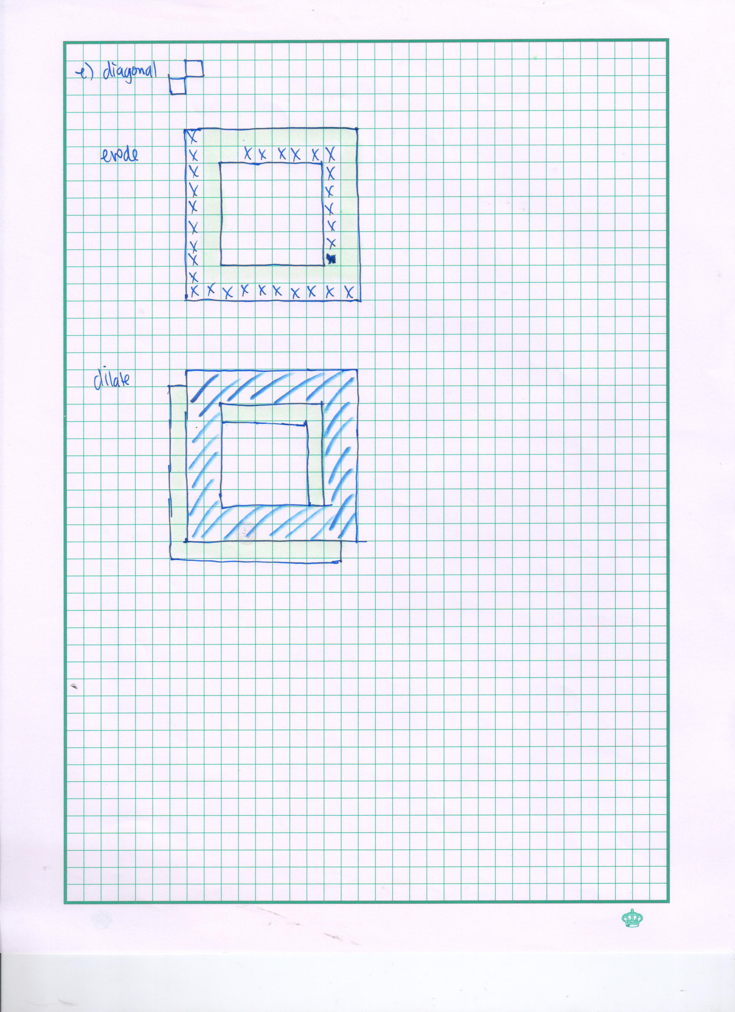
To get a better grip on the concept of the morphological operations, I draw these shapes and predicted their results after erosion and dilation on a graphing paper. The results I obtained is shown in 5 images below.

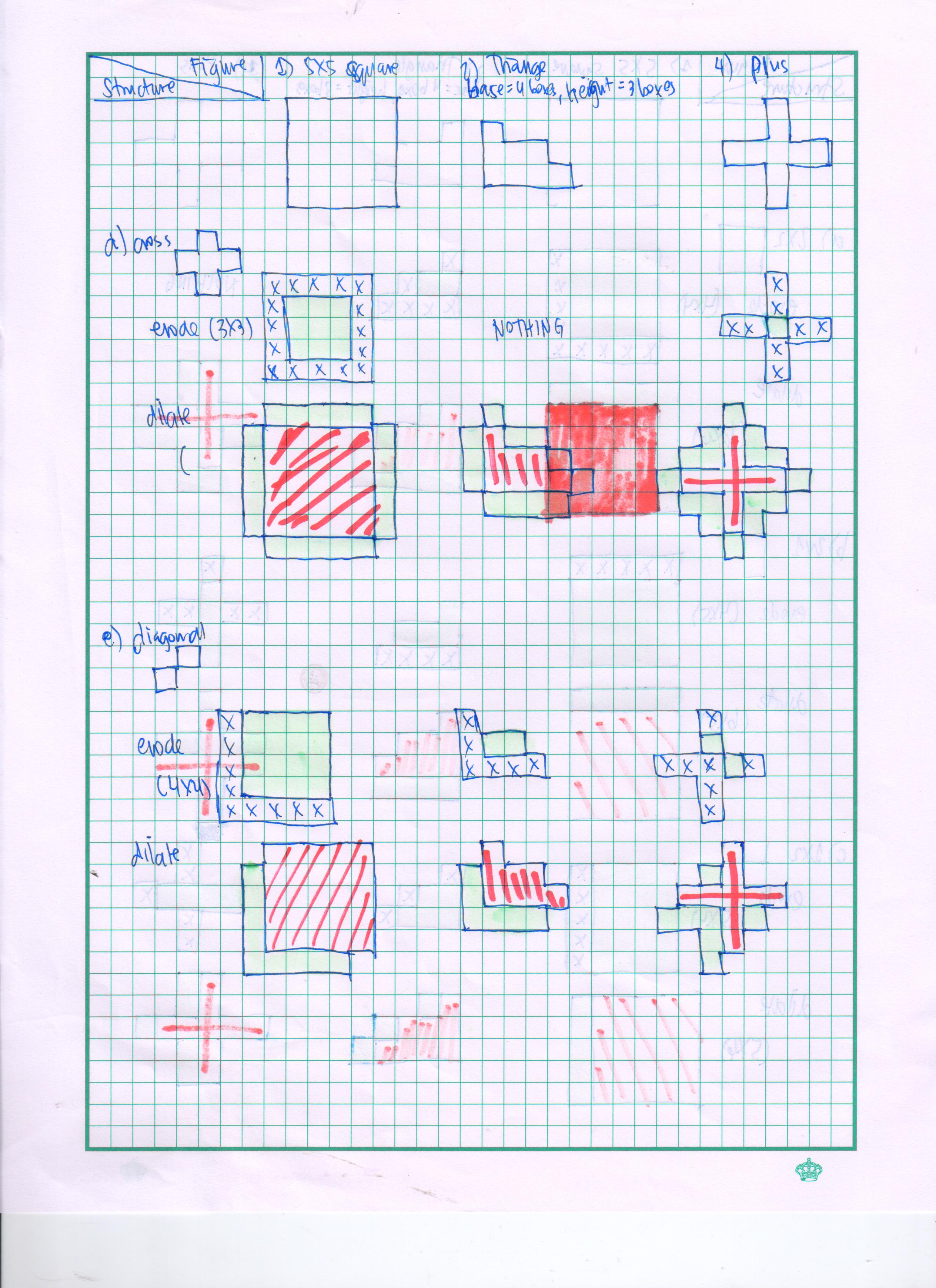
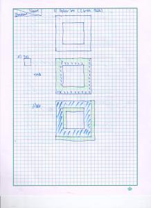

To check my predictions, I used the Image Processing Design (IPD) module of Scilab. I performed the morphological operations to each binary shape for each structuring element. The results are as follows for the 5×5 square, triangle, hollow box and a plus sign respectively.
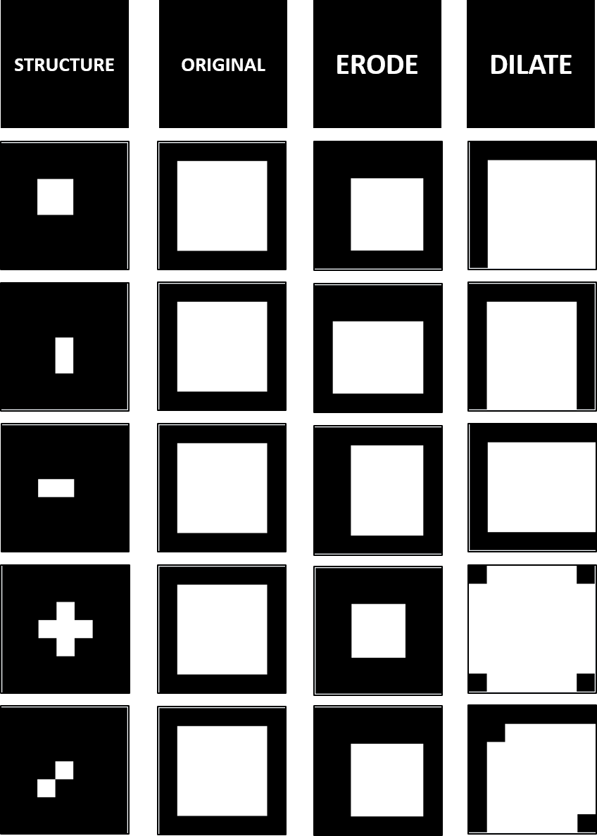
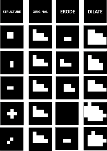
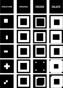
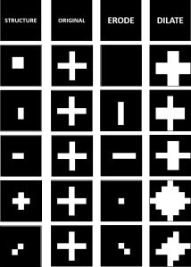
Comparing my manual prediction to the results in Scilab, I believe I had a better understanding of the concepts of erosion and dilation. I obtained the same results for each figure. As we can observe, in erosion, a pixel is eroded if the structuring element is not fitted in the binary image. That is, if the structuring element is placed in the pixel and not all pixels of the structuring element is an element of the binary shape, the certain pixel is eroded or zeroes out. In dilation, if the structuring element is not fitted in the binary image, the binary shape is expanded following the shape of the structuring element.
Application
After observing and discussing erosion and dilation, we observe three other morphological operations: Open, Close and TopHat. These morphological operators are a product of the erosion and dilation of binary images. We further discuss these operations.
Open operation involves preserving the foreground regions that have a similar shape to the structuring element while eliminating all the other regions of foreground pixels. In simple terms, the open operation is defined as an erosion followed by a dilation using the same structure element. Simply, open = dilate(erode(shape, element), element).
Close operation is a dual of opening. It involves preserving the background regions that have a similar shape to the structuring element while eliminating all other regions of background pixels. In simple terms, the close operation is defined as a dilation followed by an erosion using the same structure element. Simply, close = erode(dilate(shape, element), element).
TopHat transform is also called the peak transform. A binary image applied by an open operator by a structuring element is subtracted from the original image. The brightest spots on the original image are highlighted using this transformation. In simple terms, tophat = shape – open(shape, element).
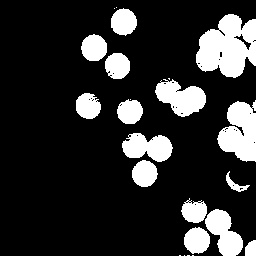
To observe these operations, we used them in a simple application of these operations. A well known application of the morphological operations is the identification of cancer cells from normal cells. We simulate this application using the figure below. It shows “cancer cells” (bigger cells) joint along the “normal cells” represented by punched paper bits.
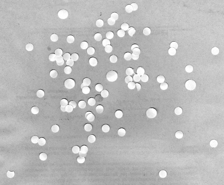 To perform the identification of cancer cells, we first examine the normal cells. We aim to know the area of the normal cells to isolate them with the cancer cells. We use the image below to calculate the approximate area of the normal cells.

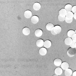
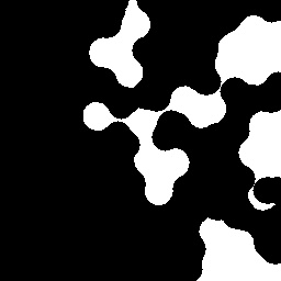
To have a better approximation of the area, we divide the original image into 10 subimages of size 256×256. We would be able to get more data points and have a better calculation of the area of a normal cell. We apply the open, close and tophat operators to a subimage to observe the effects of these operators. The structural element used is a circle of radius 12. The subimage used and its grayscale version are shown below.
Open operator:
Close operator:
TopHat operator:
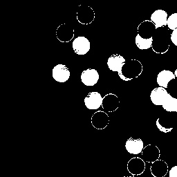
We can observe in the grayscale version of the subimage used that it still has unwanted white spots that are not part of the “normal cells”. The normal cells are also not “whole” in the sense that there are missing parts of the circle. Using the morphological operators, we observe some things. The open operator clearly removes these white spots and made the “normal cells” whole. The close operator connects the cells and distorts the image by doing so. The tophat operator as defined subtracts the image produced by the open operator to the original image. By these results, we opt to use the open operator to identify the cancer cells.
Now that we have the operator to use for our cause, we first approximate the area for the normal cells. We apply the open operator for the 10 subimages using a circular structuring element. We search for blobs using the SearchBlobs command of the module of Scilab. It automatically label each blob and calculate each area in terms of number of pixels. After obtaining the area of each blob, we plot the histogram of the number of blobs with the blob area. The histogram is shown below.
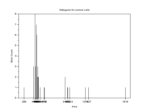
Most of the normal cells are in sizes between 300-600 square pixels. Areas below are small enough to be considered normal cells. Clump of cells are the ones with areas greater than 600 square pixels. We get the mean area using these values. To have a flexibility of the approximate area, we also calculate the standard deviation for the area of the cells. Now we have an approximate area for our normal cells.
We move on with the image with the cancer cells and normal cells. We apply the open operator with the grayscale version of the image by a circular structuring element with radius 13. We label the blobs with the same command and created a size histogram shown below.
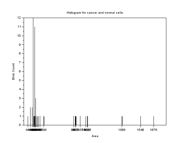
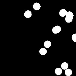
After applying the open operator, we can observe in the histogram that the normal cells are the ones with the area less than 600 square pixels. A group of peaks greater than this value can be considered as the cancer cells and some clump of normal cells. We remove these normal cells by taking into consideration the blobs with areas within the range of (mean area – standard deviation) to (mean area + standard deviation). We also remove the clumps of normal cells. The resulting image is shown below.
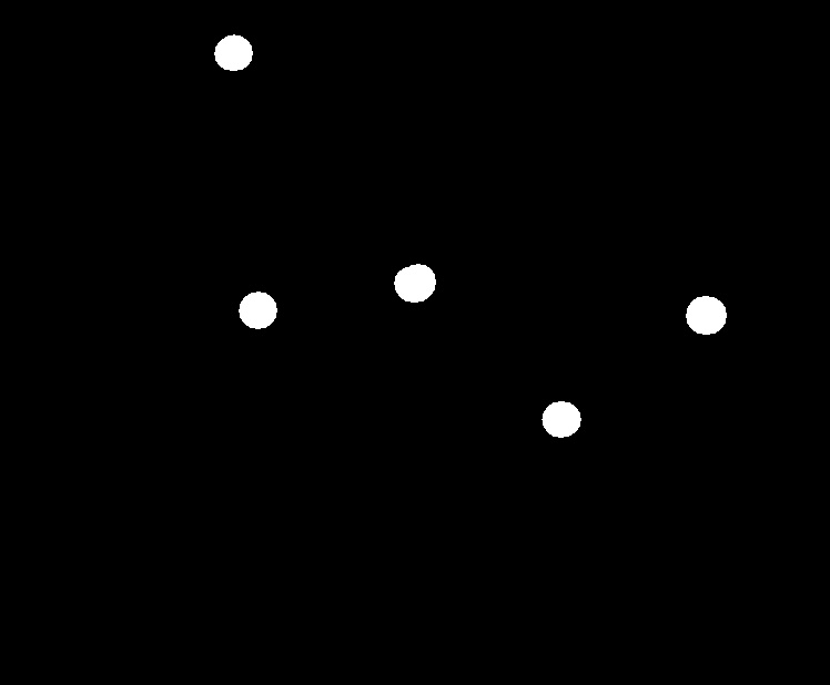
We were able to isolate the cancer cells using the open operator and the size histogram. In this way, we see the application of the morphological operations in identifying cancer cells from normal cells. From the original image, we could already identify the cancer cells. We successfully isolated the cancer cells.
Review and Self-Evaluation
I was able to learn the concepts of morphological operators. Applying these operators, we were able to observe a well known application of the morphological operators. The “cancer cells” in the image were identified and isolated to the “normal cells”. Because of these factors I would give myself 10 points for being able to follow instructions and present my results in an organized manner. I was not able to have another activity beyond the given instructions so I would not deserve some bonus points.
Overall, I would like to thank Jaime Olivares for providing some graphing paper during the activity, Ron Aves, Ralph Aguinaldo and Gio Jubilo for helping me sort out some issues I had with the activity. Thank you to Dr. Soriano for her continuous patience on us.
References:
- A8 – Morphological Operations, Dr. Maricor Soriano, Applied Physics 186 Manual
- http://homepages.inf.ed.ac.uk/rbf/HIPR2/open.htm
- http://homepages.inf.ed.ac.uk/rbf/HIPR2/close.htm
- http://www.inf.u-szeged.hu/ssip/1996/morpho/morphology.html

One thought on “Activity 8 – Morphological Operations”