Month: October 2015

Activity 7 – Image Segmentation

Image segmentation. We would not manually cut desired parts of the image since that would require too much work. Instead, we would use the concept of image segmentation to separate different desired parts of the image such as colors. The process requires the binarization of the image through a threshold that would be set for the image.

For a certain region of interest, we would separate this region and the parts of the image which contains the same properties and isolate them. The binarization process converts the colored image into an image composed of black and white. Upon isolation, it is upon us on what to represent the isolated parts of the image. To give us a good look, we observe an example.

Grayscale Image Segmentation

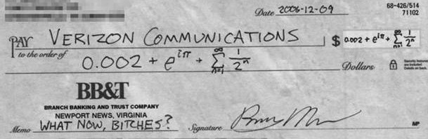
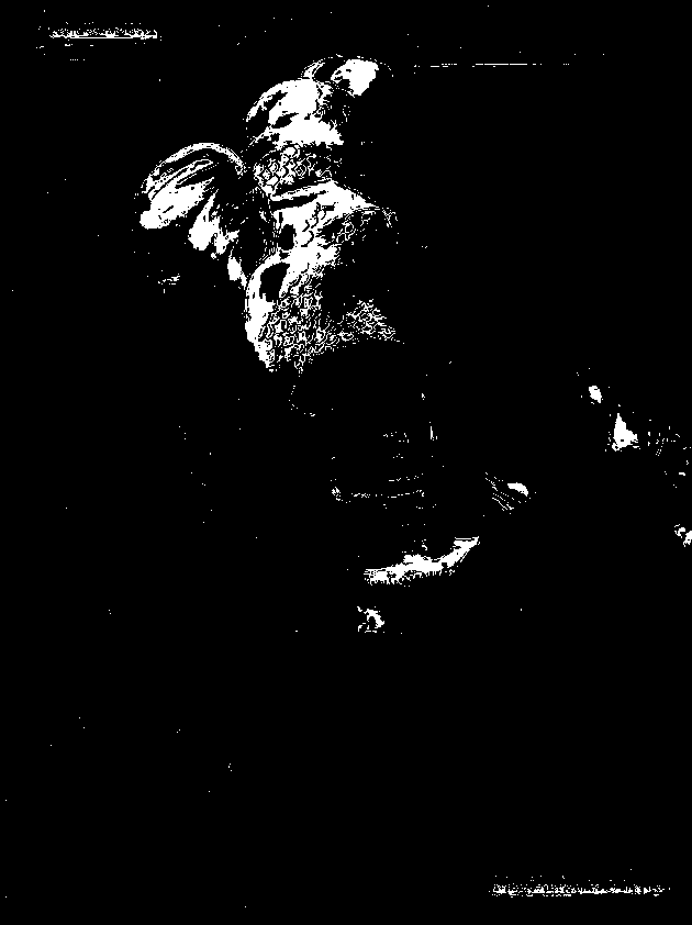
We considered a check in grayscale. Suppose we desire to isolate the hand writings and computer generated scripts in the check, we refer to the Scilab code given from the manual.

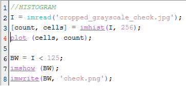The code starts by investigating on the histogram of the grayscale image. The histogram would tell us the details about the pixel values of the grayscale image. The histogram can be seen below.The peak location in the histogram corresponds to the background of the check. We can infer that they cover a lot more space than the text in the check. By choosing a threshold of 125 as shown in Line 6 of the code, we could separate the text completely from the background. The result can be seen as follows.

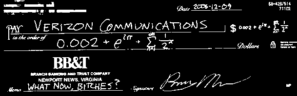
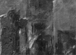
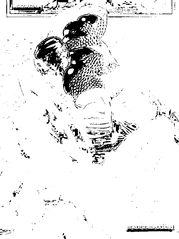
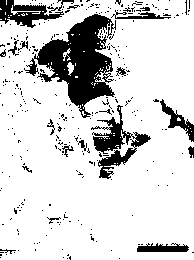
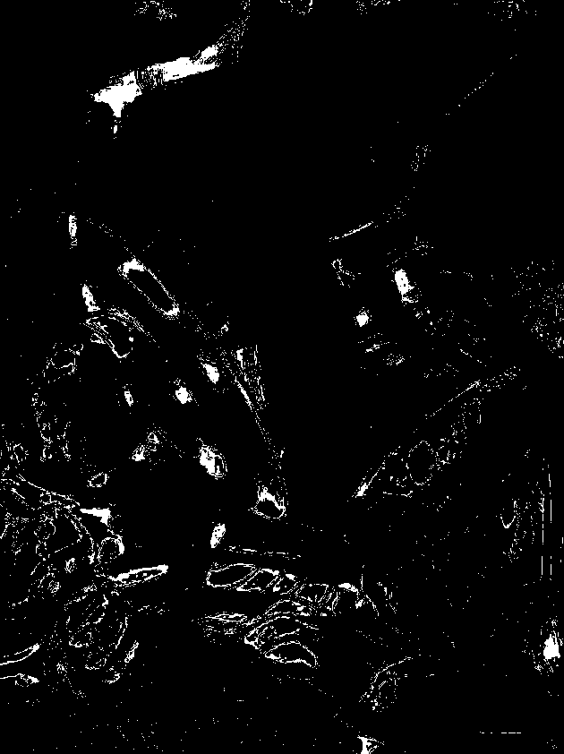
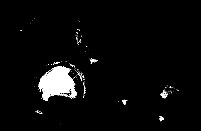
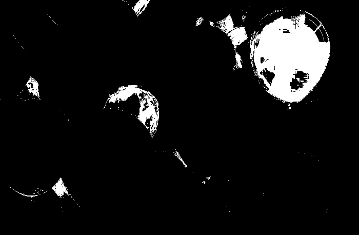
The result clearly shows that we have segmented the text from the check. We can also try different thresholds to observe if we could improve more on our segmentation. This is the case for grayscale images but as can be seen in the image below, it does not always work this way.

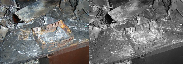
Because of this tragedy, we consider color segmentation for our images. Color is one good parameter to consider to separate regions of interest from the image. It has long been used to segment images of skin regions in faces, and
hand recognition, land cover in remote sensing, and cells in microscopy [1].

For this reason, we should consider a representation of the color space. We also need to consider the shading variations in different images where shadows darkens some colors but knowing the image, we could observe the same color for two regions. To disregard this minor problem, we would consider a color space that can separate brightness and chromaticity information [1]. This color space is the normalized chromaticity coordinates or NCC.

We first normalize the RGB coordinates by this way,

$r = \frac{R}{I}$ , $g = \frac{G}{I}$ , $b = \frac{B}{I}$

where $I = R + G + B$ . We can take note that $r + g + b = 1$ . We further simplify the coordinate system by setting the dependence of the blue channel with red and green channels, $b = 1 - r - g$ . We then can represent chromaticity with just two coordinates, r and g. The variable I would contain brightness information. The NCC can be seen as such.

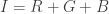
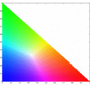
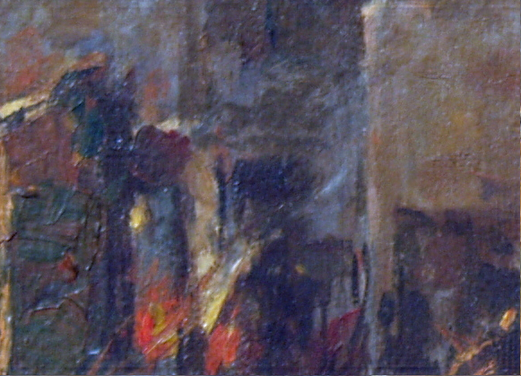
We clearly can see the dependence of the blue coordinate with the other two. When both r and g are zero, b =1 which is still consistent with the unity of all coordinate channels. Two methods of image segmentation are presented for this activity. For both activity we would try to segment the following images.

Civil War comic strip obtained from http://www.vox.com/2014/10/14/6973309/robert-downey-jr-captain-america-3-movie

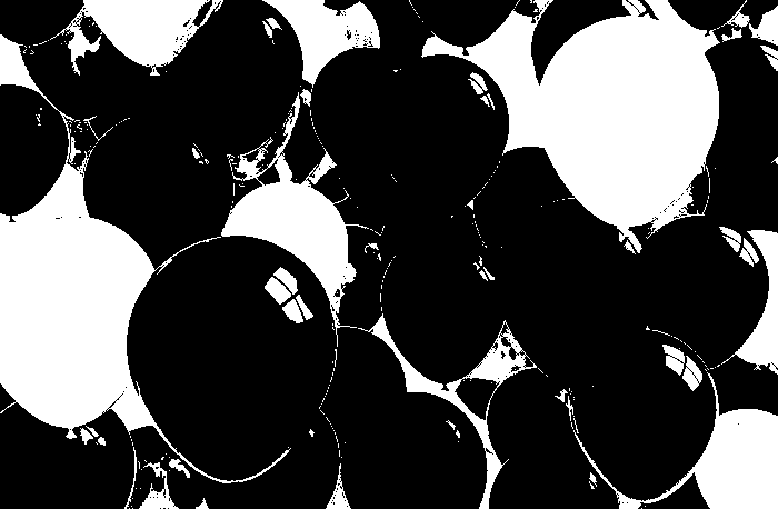
Obtained from http://polygonblog.com/3d-birthday-balloons-in-3ds-max/

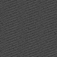
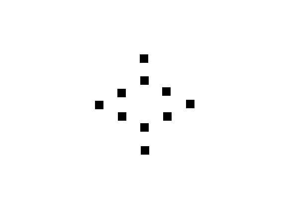
The patches considered for each images for the whole activity is given below.

The top set of 2 patches were used for the Civil War (CW) image while the bottom set of 4 patches were used for the Balloon (B) image.

Parametric Segmentation

In parametric segmentation, we consider a color distribution of interest to determine the probability of a pixel belonging to the region of interest. We first crop a region of interest and observe the histogram of the region of interest. Since we are considering the NCC, we would find the probability that a pixel belongs to the region of interest (ROI) by finding the probability that the pixel belonging to the color of the ROI. We consider both probabilities for the red and green coordinates of our NCC. The probability that the pixel belongs to the ROI is given by the equation,

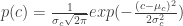
$p(c) = \frac{1}{\sigma_{c}\sqrt{2\pi}}exp(-\frac{(c - \mu_{c})^2}{2\sigma_{c}^{2}})$

where c is the color red or green. $\mu$ and $\sigma$ are the mean and standard deviation from the pixel samples. To tag a pixel as belonging to the ROI, we would consider the joint probability, $p(r)p(g)$ .

The simple code used for the parametric segmentation of the two images is shown below.

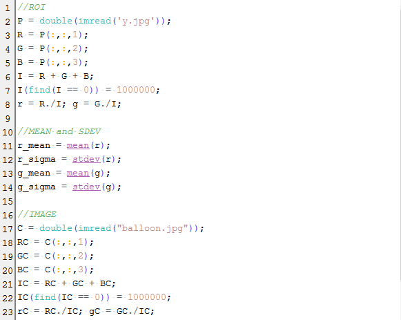
We first converted the RGB coordinates of the ROI into the NCC in Lines 1-8. The mean and standard deviations of these coordinates were calculated in Lines 10-14. The RGB coordinates are also converted into the NCC in Lines 16-23. The joint probability distribution is obtained in Lines 25-30. We placed different thresholds to observe image segmentation. Upon applying the code, we look into results of parametric segmentation in 2 images considered.

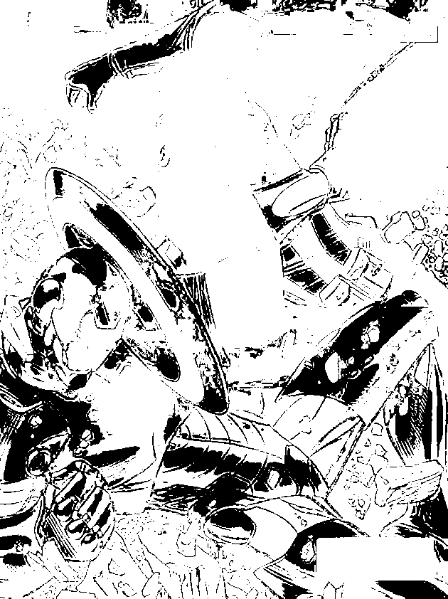
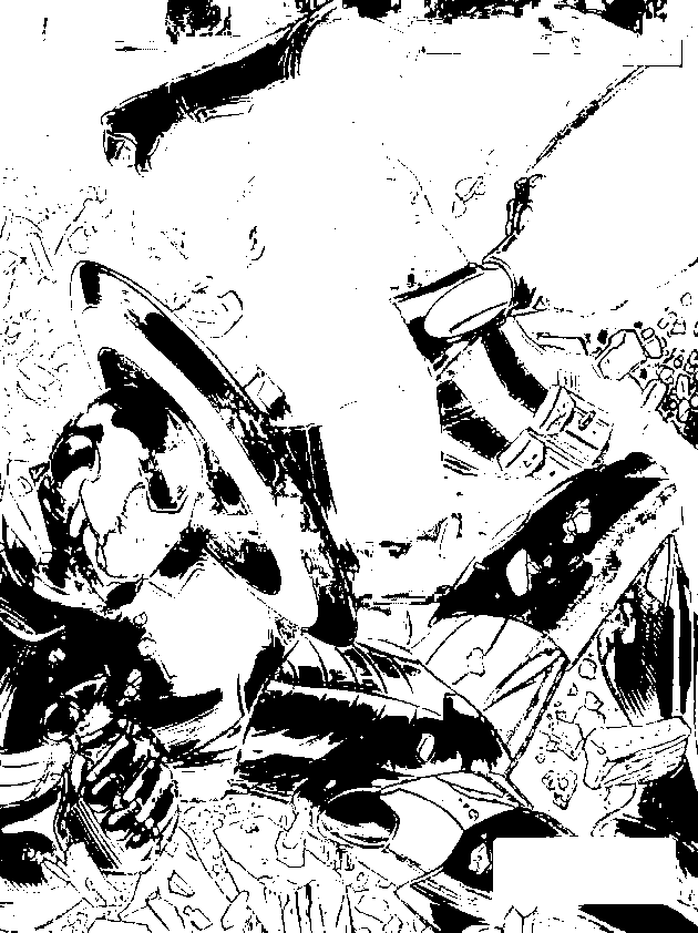
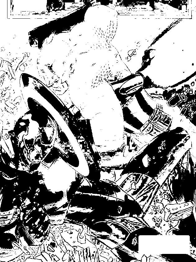
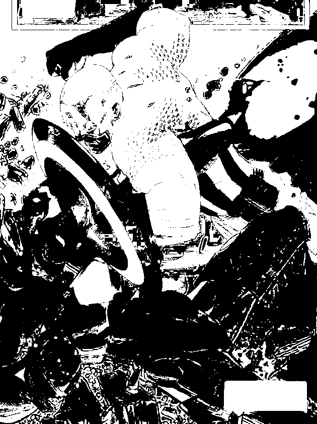
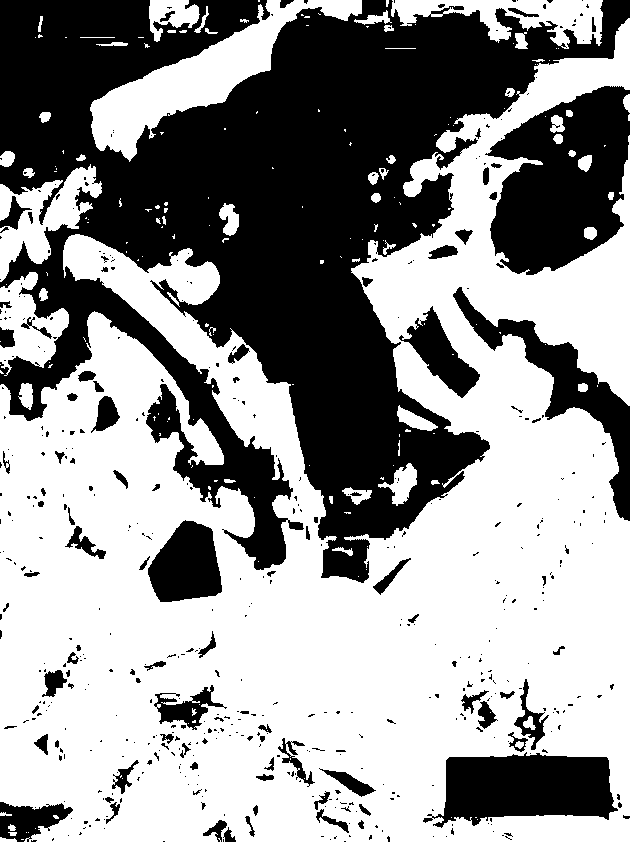
The CW image was segmented using the blue patch as ROI. Segmentation with different thresholds ranging from 0.75 – 0.95 with increments of 5 were produced. As we can observe the higher the threshold, the better segmentation we can obtain. The last image proves the power of segmentation, clearly isolating the blue uniform and some parts of the shield of Captain America. It was an awesome piece of art for me since through simple calculations of probability distributions, we can segment the some regions of an image. For the red patch, we obtain the following results,

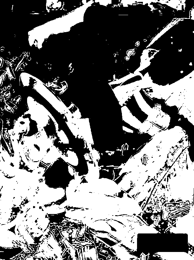
The CW image was segmented using the red patch as ROI. Segmentation with different thresholds ranging from 0.75 – 0.95 with increments of 5 were produced. The same kind of results were obtained, noting that the last image clearly isolates the red steel of Iron Man.

For a fun kind of segmentation, I had fun in the next image considered. Some results are as follows.

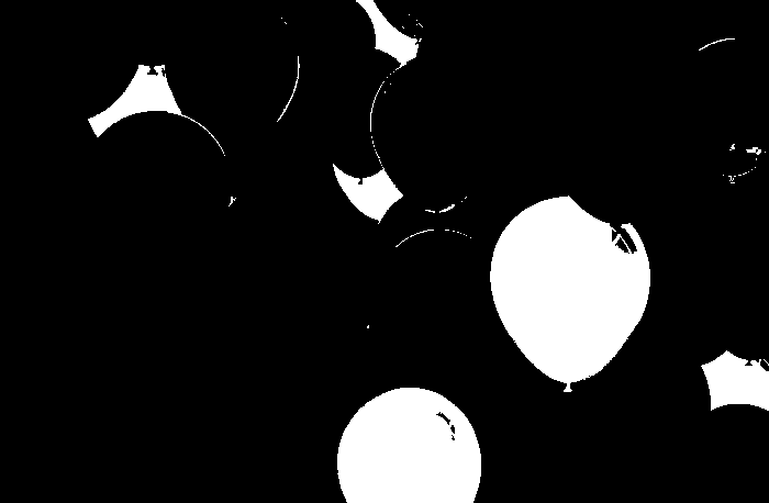
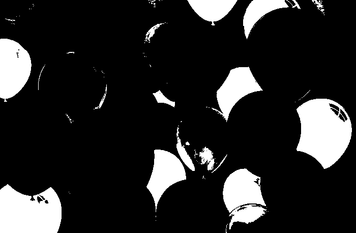
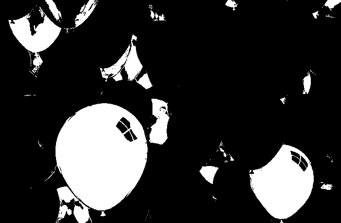
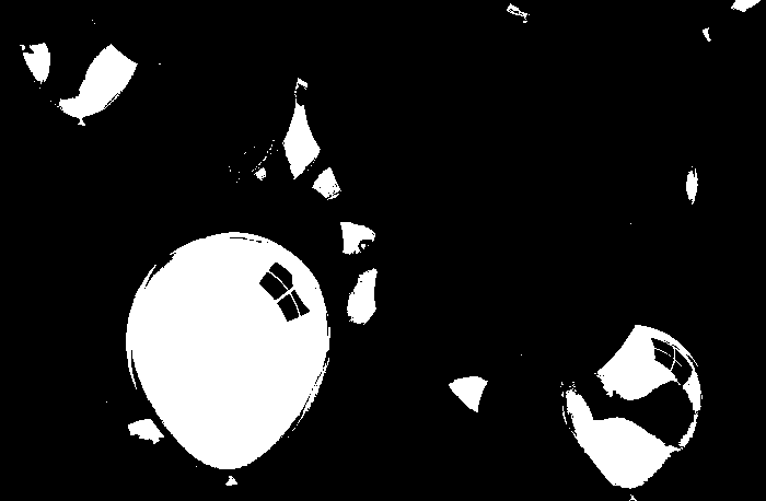
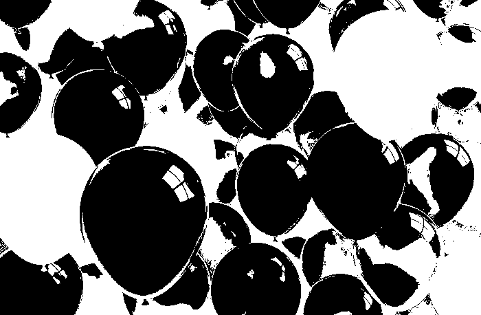
From left to right for all sets of results, the thresholds considered are 0.90 and 0.95 respectively. The first two sets used a patch of blue. There was a big difference in the two results. Referring to the original image, we can clearly choose that the right result is the one with the threshold of 0.95. The other result considered the purple balloons as part of the region of interest which we can forgive since blue and violet are colors which are close to each other.

The next two sets used a green patch as ROI. Both results are favorable but the image with a threshold of 0.90 considered the blue green balloons to be part of the ROI. But thresholds were used to eliminate some of these mistakes.

The 3rd set used a red patch as ROI. With threshold of 0.9, the returned image considered some orange balloons as part of the ROI. But then with the threshold raised to 0.95, only red balloons were considered. This set was the best set for me since I was amazed that the algorithm used denied the entry of the window-like shadow and some reflection in the right most red balloon.

The 4th and last set used a patch of yellow for ROI. For both results, orange balloons were considered. Somehow even with a high threshold, some of these errors occurs. I believe that changing and being careful of choosing the ROI could avoid this kind of mistakes.

Overall, the method of parametric segmentation proves to be a good and accurate choice for image segmentation. Though we could note that for larger sizes of image, a larger processing time would be expected. These are some important factors we need to consider for choosing our method of image segmentation in the future.

Non-parametric Segmentation

In parametric segmentation, we basically fit an analytic function to the histogram to create a function in checking if the pixel of an image belongs to the ROI. But the method’s accuracy depends solely on the goodness of the fit of the probability distribution function considered.

In the non-parametric segmentation, we use the histogram itself to admit the pixel as member of the ROI. A technique called histogram backprojection is necessary to perform non-parametric segmentation. Histogram backprojection tells us that basing on the color histogram, every pixel location is given a value equal to the histogram value in chromaticity space [1].

We first convert the r and g chromaticity coordinates into integer values and binning the image values in a matrix. The technique of histogram backprojection is shown in snippets of code below.

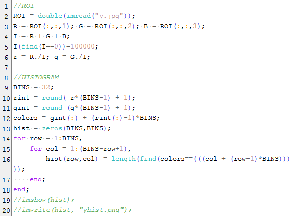Lines 1-6 converts the RGB components into chromaticity coordinates. The 2D histogram was made in Lines 8-18. The r and g values were first converted into integers and then binned these image values in a matrix.

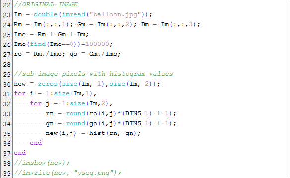
The RGB values of the original image was converted to chromaticity coordinates in Lines 22-27. The process of histogram backprojection can be seen in Lines 29-37. In Line 35 the pixel location is given a value equal to its histogram value in chromaticity space. To better understand this concept, let’s discuss the results.

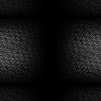
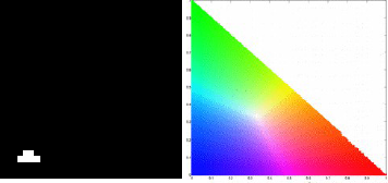
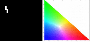
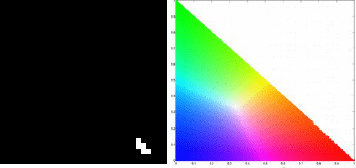
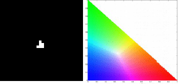
For the CW image, we obtain the following histogram for our patches. The first histogram is for the blue patch and the bottom histogram pertains to the red patch. The NCC image is shown next to the histogram to properly locate the locations of the color of the patches considered.

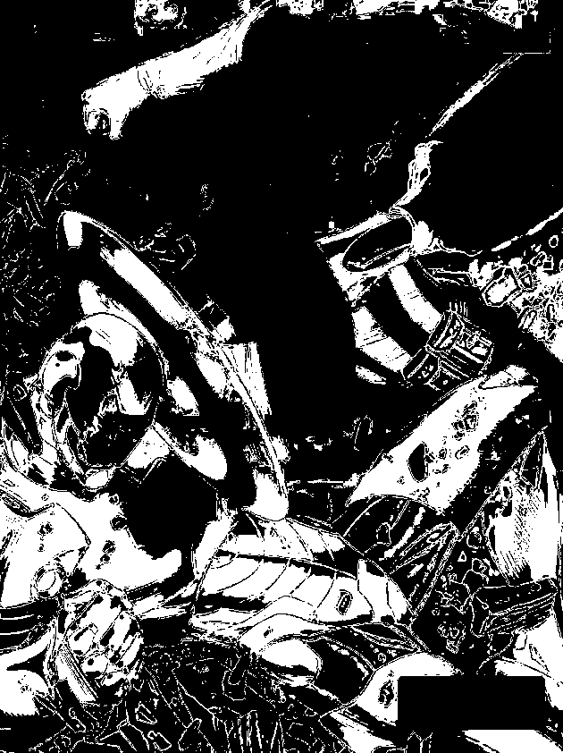
We can clearly confirm the correctness of the histogram obtained for both patches. These histogram serves as the basis for our new pixel values of the original CW images. Performing histogram backprojection to the CW image, we obtain these results.

The middle image is the result of the non-parametric segmentation of the original image (left most image) for the blue patch. The last image is the result for the red patch. For the blue patch, we can clearly observe the isolation of the blue color of the uniform of Captain America. For the red patch there are some parts that were not segmented. These results proved that the patch used for segmentation matters so much. I feel that if I replace the patch with a better patch, I would obtain much better results.

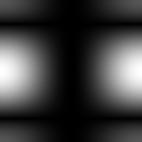
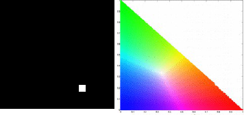
For the balloon image, I obtained the following histograms for the following patches: blue, green, red and yellow respectively.

We obtain correct histograms for the patches. The results of non-parametric segmentation of the balloon image for each patch is shown below.

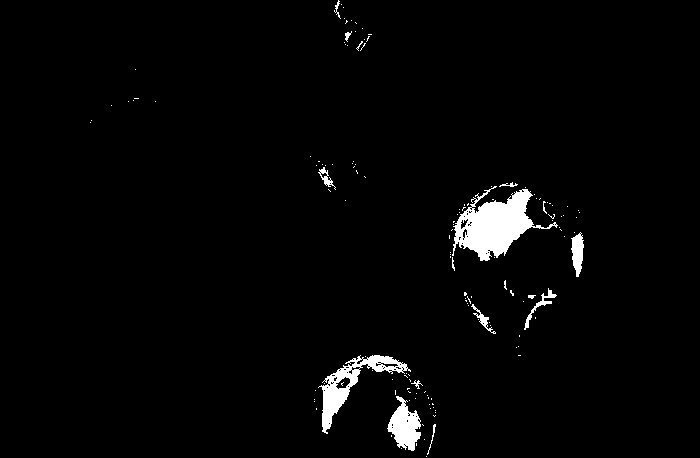
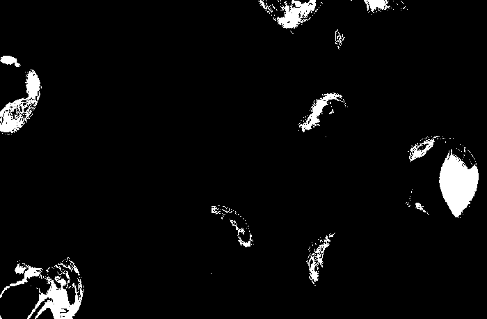
Again I believe that improving the patches considered for segmentation, we can have better results. The patches might be uneven or worse, a shade darker or lighter than most of the colors of the images.

Non-parametric segmentation is a more flexible method compared to the parametric method. Because we consider histograms, we could define ROI’s of multiple colors and still effectively segment the image. The parametric segmentation has the limitation of having an ROI of only a single color. Non-parametric segmentation also has a faster processing time since it involves no computation. The 2D histogram contains more reliable information for the pixel values we aim to segment.

After finishing the activity, I felt more skillful in image processing. A new skill such as what we gain in this activity is overwhelming. I just know that somewhere and sometime I would be able to use my new gained skill. I had lots of fun in this activity. I was amazed by my results. I am in awe of how simple the process could be to segment the images with the desired ROI. Soon I’ll add some more results which I would be able to do on some leisure times. I already have ideas on mind and I hope it would bear fruit.

Overall, I give myself 10 points for this activity because I believe I was able to do what is asked. The results I obtained are great and clearly what were asked for. Since I was not able to go beyond what is asked for, I do not deserve some extra points. If anything else, I gained lots of new skills due to these strings of activities we have for AP 186. Thank you Maam for being patient with us through these activities.

PS. I would like to thank Ron Aves, Gio Jubilo and Ralph Aguinaldo for giving me some insights on some parts of the activity.

Reference:

A7 – Image Segmentation, Applied Physics 186 Activity 7 Manual, Dr. Maricor Soriano

Activity 6 – Properties and Applications of the 2D Fourier Transform

In Activity 5, we explored the properties of Fourier transform and the convolution theorem. This time we examine the properties of the 2D Fourier transform and its applications. With more familiarity with the discrete FFT, we expect that we can have some ease with this activity. Though the workload for this activity is much heavier, it provides us with more fun challenges not to undermine the real and awesome image processing skills we expect to obtain from these activities.

Anamorphic Property of FT of different 2D patterns

According to the Merriam-Webster dictionary [2], “Anamorphic” means producing, relating to, or marked by intentional distortion of an image which tells us the kind of results we aim to produce for this part of the activity. Let’s recall that the FT space is in inverse dimension to the original space. We can also recall that what is wide in one axis will be narrow in the spatial frequency axis. This is the anamorphic property of the Fourier transform [2]. Different dimensions along each axis results into anamorphism along each axis independently. We examine the anamorphic property of the Fourier transform.

A tall rectangle aperture is observed as shown in the upper leftmost image. Its shifted FT is shown next to it. As expected a quadrilateral aperture has an FT of a cross like fringe patterns. The bottom image is a zoomed in version of the mat2gray shifted FT of the tall rectangle aperture. The FT shows anamorphism since we can observe the distortion in the image axes. We have a tall rectangle aperture which is wide with respect to the y-axis but we can observe the middle fringe pattern to be wide in the x-axis. To further observe this property of the FT, we observe the wide rectangle aperture.

We can observe anamorphism in the FT of the wide rectangle. The wide rectangle is wide in the x-axis but the middle fringe pattern shows favor in the y-axis. The distortion shows this common property of the Fourier transform.

dot_2

We produce an image of two dots from the center along the x-axis symmetric about the center, both 2 pixels away from the center. This constitutes somehow a double slit for our interference patterns. As expected the FT of this figure are fringe patterns. It is also wide in the y-axis as anamorphism suggests. Changing the spacing between the dots produces such results,

dot_10

The dots are placed 10 pixels away from the center. There are more fringe patterns along the x-axis. The spacing between the dots determines the frequency of the corrugated roof pattern. 5X spacing produced 5X more frequency for the FT fringe patterns.

Rotation Property of the FT

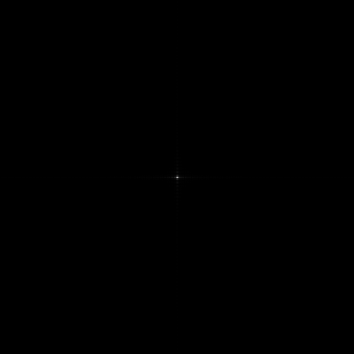
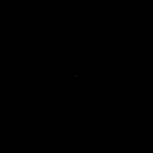
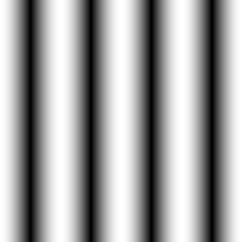
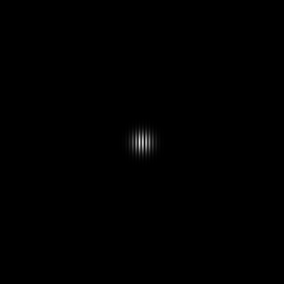
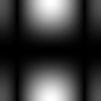
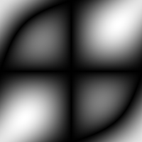
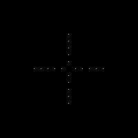
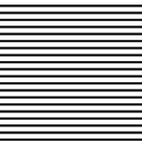
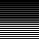
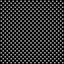
From anamorphism, we observe the rotation property of the Fourier transform. The best way to observe this is through synthetic images of a sinusoid through a corrugate roof pattern. Given the example code in the manual, a synthetic image of a sinusoid in the x-direction was produced. The sinusoid is in the form $sin2\pi f X$ where f is the frequency. Its FT was obtained and the FT modulus was displayed. With a frequency of 4, the sinusoid and its FT is shown below.

unsurprisingly, the FT of the corrugated roof in the x-axis turns out to be two dots arranged in the y-axis. Anamorphism is again shown in this result. When we change the frequency of the corrugated roof pattern, we observe these results.

Fz4

The images of the sinusoid (top) with their corresponding FTs (bottom) are placed in increasing frequency. We can observe that as we increase the frequency of the corrugated roof pattern, the spacing of the two dots to the center along the y-axis is increased. Since digital images don’t have negative values, there is a need to add a bias to our sinusoids to produce real images. Adding some constant bias, the FTs of the corrugated roof in increasing frequencies is shown below.

The pixel in the middle represents the bias I added in the sinusoidals. As we increase the frequency, the spacing between the dots increases as well. So if we take an image of an interferogram for a Young’s double slit experiment, we can find the frequency of the fringe patterns produced by simulating and taking the FT of two dots with the same spacing of the slits in the experiment. From this experiment, we expect to observe a sinusoid and its frequency is the same as the fringe pattern we observe in the actual experiment.

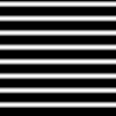
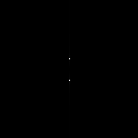
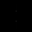
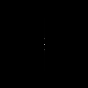
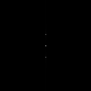
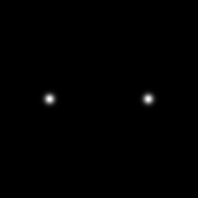
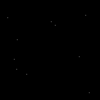
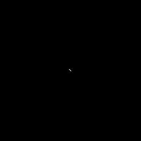
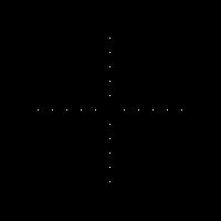
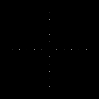
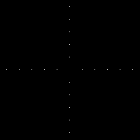
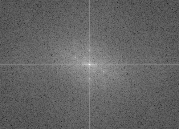
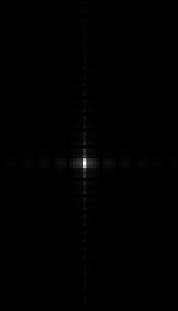
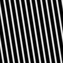
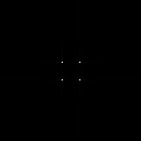
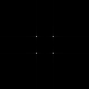
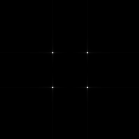
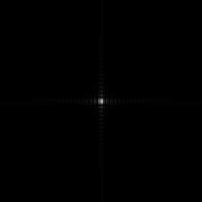
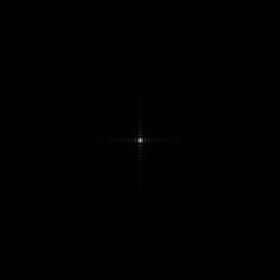
Suppose we add a non-constant bias in the form of a very low-frequency sinusoidal of the form $sin0.4\pi X$ , we obtained the following results. We can observe the spacing of two dots increases as the frequency of the original sinusoid is increased. We can also observe another set of 2 dots in the middle which can be attributed to the very low frequency added. So for an interferogram setup where a non-constant bias is added, we still can determine the frequency of the interferogram by simulation and the use of Fourier transform.

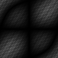
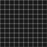
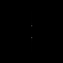
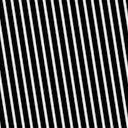
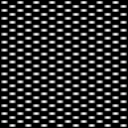
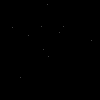
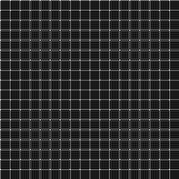
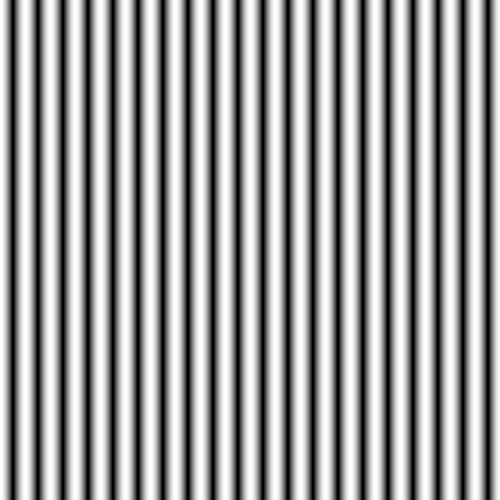
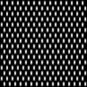
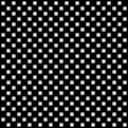
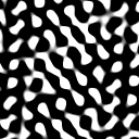
Rotating the original sinusoid by $30^{o}$ , the new sinusoid form is in the form $sin(2\pi f(Y*sin(\theta) + Xcos(\theta))$ . The resulting images and their FTs for different frequencies is shown below.

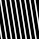
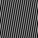
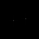
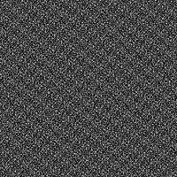
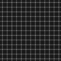
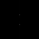
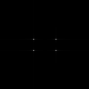
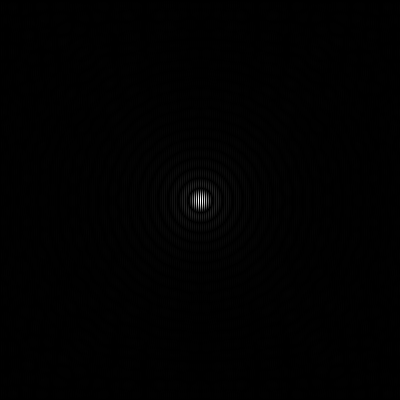
As observed in previous results, increasing the frequency also increases the spacing between the dots. The FT was also rotated by the same angle as the original image. The rotation property of FT is manifested in these results. The amount of rotation we imply on an image is the same rotation that is implied in its FT.

A combination of two sinusoids of the form $zc = sin(2\pi fX) sin(2\pi fY)$ in different axes and their resulting FTs are shown below.

The spacing between the dots in the FT remain dependent of the frequency of the sinusoid in the axes. We may consider two dots to be one unit and the spacing between the sets of dots are dependent of the frequency of the sinusoid. The results are shown in increasing frequencies in sinusoids in the x-direction with different frequencies in the y-direction.

Combining all the results we gather, I ended up adding several rotated sinusoids to a combination of sinusoids in the previous set of results. The resulting image and its FT is shown below.

zcr

With a combination of two sinusoids and the addition of several rotated sinusoids, we can clearly observe the rotation property of the FT where several rotated FTs and the spacing between the dots occurred in the FT of this abstract image in the left. It is quite amazing how we played with this part of the activity and ended up producing such results. I had so much fun in this part of the activity.

Convolution Theorem Redux

To start this part of the activity, two dots are placed along the x-axis symmetric about the center. From previous results, we know that the FT of this image is a corrugated roof pattern. We add some twist with this activity to further observe the convolution theorem.

Instead of dots, circles were placed symmetric along the x-axis. The FT of the image was taken and observed in different radius of the circles. The results are as follows.

Fcircles2

And voila! In my delight, the results are so good. From the previous blog post, we can recall that the FT of a circular aperture is a Poisson pattern. Placing two circular apertures symmetric about the center much like a double slit setup does not only produce a Poisson pattern but also a fringe pattern enclosed in the Poisson pattern! Such a beauty! We can also observe the difference of increasing radius of circles. Increasing the radius, decreases the size of the Poisson pattern observed.

We replaced the circles with squares of different widths. The FT of a square aperture is a cross like pattern with radial fringes along the x and y axis. I am so excited to see the results of this image and was not disappointed. Here are the results.

Convolution is the real thing. The radial fringe pattern was embedded with another fringe like pattern due to the presence of two square aperture. Also as we increase the width of the squares, the smaller pattern is produced.

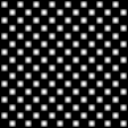
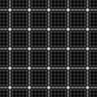
Now it gets crazier since we are bound to change the squares with Gaussians of the form $exp(\frac{-(x\pm \mu_{o})^{2}}{\sigma^2})$ of varying $\sigma$ where $\mu$ are the peak locations. The results are as follows.

Fgauss20

The FT of a Gaussian is also a Gaussian. The Gaussian produced still has fringe patterns embedded in it. The larger the $\sigma$ , the larger the size of the FT becomes.

To further observe the convolution theorem, we created an array of 200 x 200 zeroes. 10 random points were filled with 1’s. The 1’s would approximate the dirac deltas. A set of 5, 3×3 patterns were created and was convolved with the array of random 1’s. The results are shown below.

s-rand

s-afft

s-conv

The first two figures shows the array of random 1’s and the spot pattern. Their FTs are directly below their images. The left bottom most image is the convolution of their FTs. We can clearly see the resemblance of the figure with the FTs of the array and patterns. The convolution is the right bottom most image. But since the pattern considered is very small we cannot see the right image. The image supposedly features the pattern placed in the random 1’s. 10 spot patterns should be seen in the locations of the 1’s in the array. But since we can still view the FT of their convolution, we can still conclude that we obtained the right convolution of the array and the pattern. We view other patterns and random arrays.

For a vertical pattern, the results are as follows.

v-rand

For a horizontal pattern, we observe these results.

For a diagonal pattern, these are the results.

A 200 x 200 array of zeroes was made where equally spaced 1’s along the x and y axes are placed. Considering different spacing between the 1’s, the images and their corresponding FT’s are shown below.

A13

A15

A18

As we increase the spacing, we observe more “windows”. These windows are more likely produced by overlapping fringe patterns along both axis. We may also try adding more 1’s in the array and the result of its FT is the presence of more of these “windows”.

Well the main goal of this part of the activity is to show that we can filter an image through its Fourier space domain. Any unwanted repetitive pattern in an image can be filtered by masking their frequencies in the Fourier domain. We can also enhance the image by enhancing the frequencies of desired features. We will further observe this in the next parts of the activities.

Fingerprints: Ridge Enhancement

Supposedly, we are to prepare an image of our own fingerprint for this activity. I was unable to produce one due to lack of a stamping ink and lack of creativity. Honestly, this was my main problem in the activity. I was lazy enough to wait for an image of a fingerprint before I was able to move on with the activity. Luckily, I found my stride to finally search for a fingerprint in the web and found this gem.

Fingerprint retrieved from http://www.creativeclass.com/_v3/creative_class/2008/09/30/get-it-right-puh-leaze/

To properly the ridges of the fingerprint, we obtain the grayscale of the fingerprint. The FT of the grayscaled fingerprint was also observed.

fp-bin

The FT of the fingerprint gives us the idea of the filter we ought to use. We need to retain the two concentric circles in the middle and filter the rest of the FT. Filtering in the Fourier space is one of the most effective way to remove unwanted patterns. In this case, the botches are what we want to remove. The frequencies of the ridges lie on the concentric circles. The filter used is shown below.

The hardest part of making the filter is the estimation of the concentric circles that we ought to retain. When the filter was already made, we convolve the filter and the FT of the grayscaled fingerprint. The resulting convolution is shown below.

We can observe the removal of the botches and the clearer appearance of the ridges. The ridges are necessary since they make anyone’s fingerprint unique. The botches we encountered are unavoidable since there is an uneven distribution of the ink when we capture our fingerprints. Filtering in the Fourier domain provides us an easy way to process and enhance our images.

Lunar Landing Scanned Pictures: Line removal

A 1967 lunar picture is shown below. This picture was obtained by the unmanned Lunar Orbiter V spacecraft prior to the Apollo missions to the Moon. The black and white film was automatically developed onboard the spacecraft and
subsequently digitized for transmission to Earth. The regularly spaced vertical lines are the result of combining individually digitized ‘framelets’ to make a composite photograph and the irregularly-shaped bright and dark spots are due to nonuniform film development [3].

The lines are the unwanted repetitive patterns for this image. We remove this in the Fourier space. The FT of the grayscaled version of the image is shown below.

The lines along the x and y axes are the frequencies of the unwanted repetitive line patterns. We need to retain the small circle in the middle as it contains the important information of the picture. Unlike in the case of the fingerprint, we retain the other areas and just completely eliminate the vertical and horizontal lines in the axes. The filter used for the enhancement of the figure is shown below.

The circle in the middle was effectively filtered and the lines in the axes were eliminated. The resulting FT of the convolution of the filter and the FT of the grayscaled image is as follows.

lun-enhanced

The image on the left side is the product of the filter and the grayscale version of the original image. The right side is the product of the filter applied to the RGB channels of the original image. As we can see for both products, the unwanted repetitive lines are clearly removed using the filter. The method of filtering in the Fourier domain proved to be an effective way of enhancing these images.

Canvas Weave Modeling and Removal

The last part of the activity directs us to modeling a canvas weave and eventually enhancing a painting by removing the said unwanted part of the image. The image considered is shown below.

As we can observe, the image of the painting has the obvious patterns of the canvas weave. The pattern is what we aim to remove to enhance the detail of the oil painting. The FT of the grayscale version of this image is given below.

The unwanted repetitive pattern given by the canvas weave is defined by the blots in surrounding the middle area of the FT. These are the patterns we need to remove from the FT image while retaining the entire area, the lines in the axes and the circle in the middle. Using GIMP, I covered these blots using black squares. The filter produced in the process is shown below.

Applying the filter to the FT of the grayscale image of the oil painting, we obtained the FT of the convolution given by the images below.

weave-enhanced

The left side is the product of the filter and the grayscale image of the oil painting. The right image results from the application of the filter to the RGB channels of the original image. For both results, we observe that we have completely removed the canvas weave pattern. The brushstrokes are also improved as observed in the colored result. We completely enhanced the image using the method of filtering in the Fourier domain. If we inverse the filter and convolve it with the FT of the image of the oil painting, we would get the canvas weave pattern. We can therefore conclude that inversing the filter, we could obtain the unwanted repetitive patterns we removed from the images.

weave-invfilter

The activity was a whole lot of fun. I want to thank Ralph Aguinaldo, Ron Aves, Gio Jubilo, Martin Bartolome and Jaime Olivares for helping me realize some mistakes I made in my Scilab codes. They also provide suggestions most especially on the last 3 sets of activities of enhancing images by filtering in the Fourier domain. Honestly, I overthinked a lot of these activities. The activity made me realize that some things even how complicated it may seem, is just simple as saying 1-2-3. I feel like I would have completed the activity much earlier if I did not give too much time in finding ways to produce an image of my fingerprint.

Overall, the activity was both stressful yet fulfilling. Since I completed every part of the activity and produce very good results, I would give myself a 10 for this activity. I believe, I was also able to place good insights about the theories behind the results obtained for this activity. I also know that I do not deserve extra points due to the punctuality of my blog. But still, regardless of points, I feel really cool producing my results. And nobody would stop me from feeling this way.

References:

A6 – Properties and Applications of the 2D Fourier Transform, Dr. Maricor Soriano, Applied Physics 186 Manual
Anamorphic, http://www.merriam-webster.com/dictionary/anamorphic
Lunar Picture from Lunar Orbiter V spacecraft, http://www.lpi.usra.edu/lunar/missions/apollo/apollo_11/images/