In Activity 5, we explored the properties of Fourier transform and the convolution theorem. This time we examine the properties of the 2D Fourier transform and its applications. With more familiarity with the discrete FFT, we expect that we can have some ease with this activity. Though the workload for this activity is much heavier, it provides us with more fun challenges not to undermine the real and awesome image processing skills we expect to obtain from these activities.
Anamorphic Property of FT of different 2D patterns
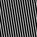
According to the Merriam-Webster dictionary [2], “Anamorphic” means producing, relating to, or marked by intentional distortion of an image which tells us the kind of results we aim to produce for this part of the activity. Let’s recall that the FT space is in inverse dimension to the original space. We can also recall that what is wide in one axis will be narrow in the spatial frequency axis. This is the anamorphic property of the Fourier transform [2]. Different dimensions along each axis results into anamorphism along each axis independently. We examine the anamorphic property of the Fourier transform.
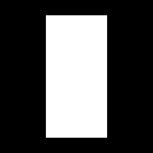
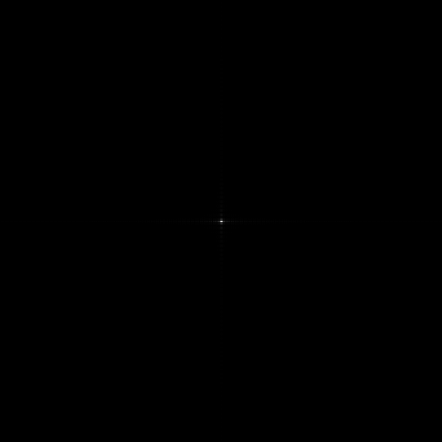
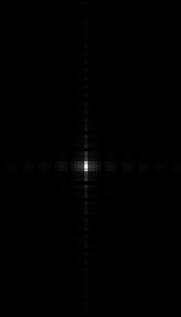
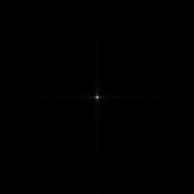
 A tall rectangle aperture is observed as shown in the upper leftmost image. Its shifted FT is shown next to it. As expected a quadrilateral aperture has an FT of a cross like fringe patterns. The bottom image is a zoomed in version of the mat2gray shifted FT of the tall rectangle aperture. The FT shows anamorphism since we can observe the distortion in the image axes. We have a tall rectangle aperture which is wide with respect to the y-axis but we can observe the middle fringe pattern to be wide in the x-axis. To further observe this property of the FT, we observe the wide rectangle aperture.


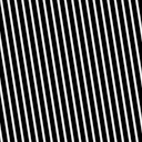
 We can observe anamorphism in the FT of the wide rectangle. The wide rectangle is wide in the x-axis but the middle fringe pattern shows favor in the y-axis. The distortion shows this common property of the Fourier transform.
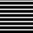
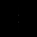
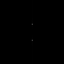
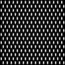
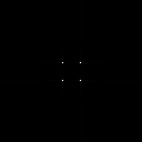
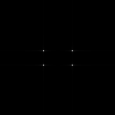
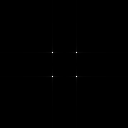
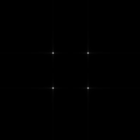
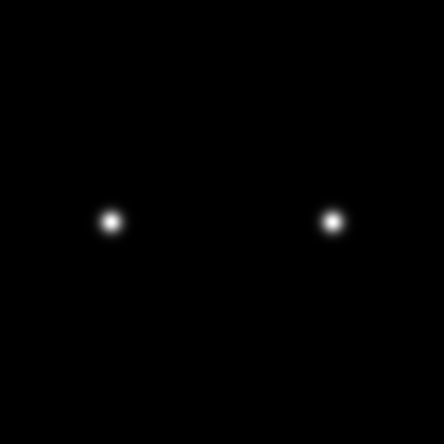
We produce an image of two dots from the center along the x-axis symmetric about the center, both 2 pixels away from the center. This constitutes somehow a double slit for our interference patterns. As expected the FT of this figure are fringe patterns. It is also wide in the y-axis as anamorphism suggests. Changing the spacing between the dots produces such results,

The dots are placed 10 pixels away from the center. There are more fringe patterns along the x-axis. The spacing between the dots determines the frequency of the corrugated roof pattern. 5X spacing produced 5X more frequency for the FT fringe patterns.

Rotation Property of the FT
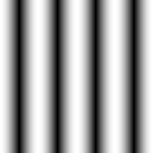
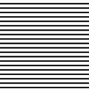
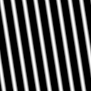
From anamorphism, we observe the rotation property of the Fourier transform. The best way to observe this is through synthetic images of a sinusoid through a corrugate roof pattern. Given the example code in the manual, a synthetic image of a sinusoid in the x-direction was produced. The sinusoid is in the form 

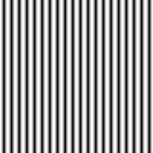
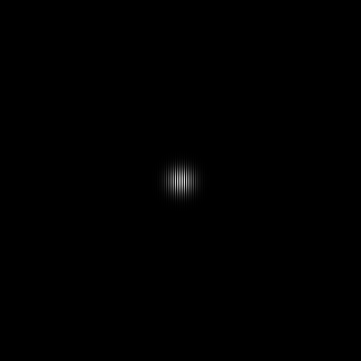
unsurprisingly, the FT of the corrugated roof in the x-axis turns out to be two dots arranged in the y-axis. Anamorphism is again shown in this result. When we change the frequency of the corrugated roof pattern, we observe these results.


The images of the sinusoid (top) with their corresponding FTs (bottom) are placed in increasing frequency. We can observe that as we increase the frequency of the corrugated roof pattern, the spacing of the two dots to the center along the y-axis is increased. Since digital images don’t have negative values, there is a need to add a bias to our sinusoids to produce real images. Adding some constant bias, the FTs of the corrugated roof in increasing frequencies is shown below.


The pixel in the middle represents the bias I added in the sinusoidals. As we increase the frequency, the spacing between the dots increases as well. So if we take an image of an interferogram for a Young’s double slit experiment, we can find the frequency of the fringe patterns produced by simulating and taking the FT of two dots with the same spacing of the slits in the experiment. From this experiment, we expect to observe a sinusoid and its frequency is the same as the fringe pattern we observe in the actual experiment.
Suppose we add a non-constant bias in the form of a very low-frequency sinusoidal of the form 


Rotating the original sinusoid by 

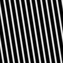


As observed in previous results, increasing the frequency also increases the spacing between the dots. The FT was also rotated by the same angle as the original image. The rotation property of FT is manifested in these results. The amount of rotation we imply on an image is the same rotation that is implied in its FT.
A combination of two sinusoids of the form 

The spacing between the dots in the FT remain dependent of the frequency of the sinusoid in the axes. We may consider two dots to be one unit and the spacing between the sets of dots are dependent of the frequency of the sinusoid. The results are shown in increasing frequencies in sinusoids in the x-direction with different frequencies in the y-direction.
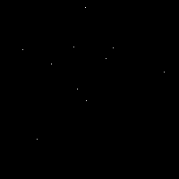
Combining all the results we gather, I ended up adding several rotated sinusoids to a combination of sinusoids in the previous set of results. The resulting image and its FT is shown below.

With a combination of two sinusoids and the addition of several rotated sinusoids, we can clearly observe the rotation property of the FT where several rotated FTs and the spacing between the dots occurred in the FT of this abstract image in the left. It is quite amazing how we played with this part of the activity and ended up producing such results. I had so much fun in this part of the activity.

Convolution Theorem Redux
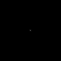
To start this part of the activity, two dots are placed along the x-axis symmetric about the center. From previous results, we know that the FT of this image is a corrugated roof pattern. We add some twist with this activity to further observe the convolution theorem.
Instead of dots, circles were placed symmetric along the x-axis. The FT of the image was taken and observed in different radius of the circles. The results are as follows.


And voila! In my delight, the results are so good. From the previous blog post, we can recall that the FT of a circular aperture is a Poisson pattern. Placing two circular apertures symmetric about the center much like a double slit setup does not only produce a Poisson pattern but also a fringe pattern enclosed in the Poisson pattern! Such a beauty! We can also observe the difference of increasing radius of circles. Increasing the radius, decreases the size of the Poisson pattern observed.
We replaced the circles with squares of different widths. The FT of a square aperture is a cross like pattern with radial fringes along the x and y axis. I am so excited to see the results of this image and was not disappointed. Here are the results.


Convolution is the real thing. The radial fringe pattern was embedded with another fringe like pattern due to the presence of two square aperture. Also as we increase the width of the squares, the smaller pattern is produced.
Now it gets crazier since we are bound to change the squares with Gaussians of the form 


The FT of a Gaussian is also a Gaussian. The Gaussian produced still has fringe patterns embedded in it. The larger the
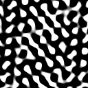
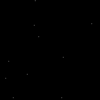
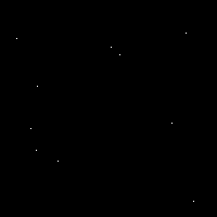
To further observe the convolution theorem, we created an array of 200 x 200 zeroes. 10 random points were filled with 1’s. The 1’s would approximate the dirac deltas. A set of 5, 3×3 patterns were created and was convolved with the array of random 1’s. The results are shown below.

The first two figures shows the array of random 1’s and the spot pattern. Their FTs are directly below their images. The left bottom most image is the convolution of their FTs. We can clearly see the resemblance of the figure with the FTs of the array and patterns. The convolution is the right bottom most image. But since the pattern considered is very small we cannot see the right image. The image supposedly features the pattern placed in the random 1’s. 10 spot patterns should be seen in the locations of the 1’s in the array. But since we can still view the FT of their convolution, we can still conclude that we obtained the right convolution of the array and the pattern. We view other patterns and random arrays.
For a vertical pattern, the results are as follows.


For a horizontal pattern, we observe these results.

For a diagonal pattern, these are the results.
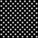
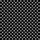
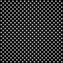
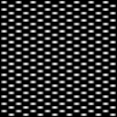
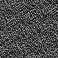
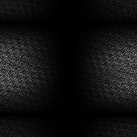
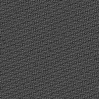
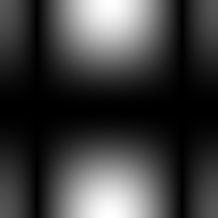
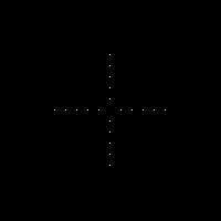
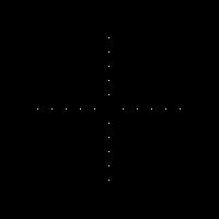
A 200 x 200 array of zeroes was made where equally spaced 1’s along the x and y axes are placed. Considering different spacing between the 1’s, the images and their corresponding FT’s are shown below.
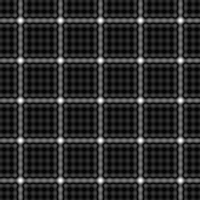
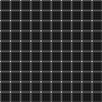
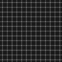
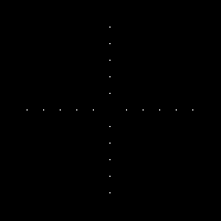

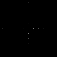
As we increase the spacing, we observe more “windows”. These windows are more likely produced by overlapping fringe patterns along both axis. We may also try adding more 1’s in the array and the result of its FT is the presence of more of these “windows”.
Well the main goal of this part of the activity is to show that we can filter an image through its Fourier space domain. Any unwanted repetitive pattern in an image can be filtered by masking their frequencies in the Fourier domain. We can also enhance the image by enhancing the frequencies of desired features. We will further observe this in the next parts of the activities.
Fingerprints: Ridge Enhancement
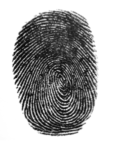
Supposedly, we are to prepare an image of our own fingerprint for this activity. I was unable to produce one due to lack of a stamping ink and lack of creativity. Honestly, this was my main problem in the activity. I was lazy enough to wait for an image of a fingerprint before I was able to move on with the activity. Luckily, I found my stride to finally search for a fingerprint in the web and found this gem.
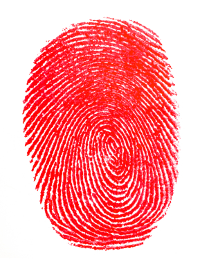 Fingerprint retrieved from http://www.creativeclass.com/_v3/creative_class/2008/09/30/get-it-right-puh-leaze/
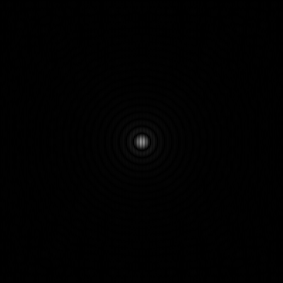
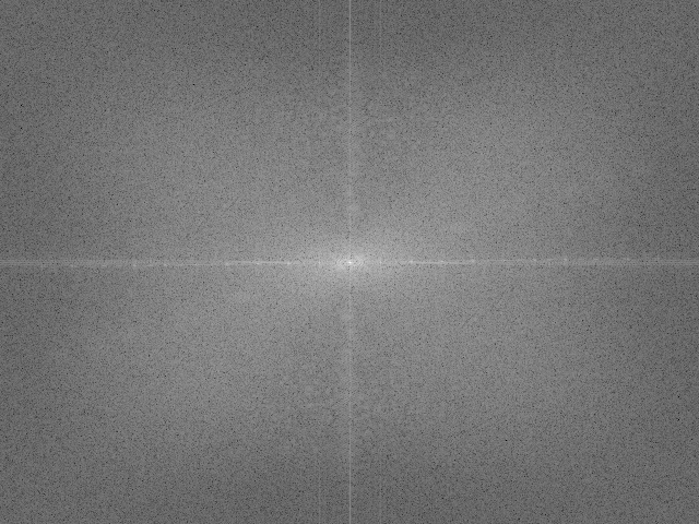
To properly the ridges of the fingerprint, we obtain the grayscale of the fingerprint. The FT of the grayscaled fingerprint was also observed.
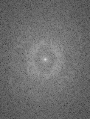
The FT of the fingerprint gives us the idea of the filter we ought to use. We need to retain the two concentric circles in the middle and filter the rest of the FT. Filtering in the Fourier space is one of the most effective way to remove unwanted patterns. In this case, the botches are what we want to remove. The frequencies of the ridges lie on the concentric circles. The filter used is shown below.
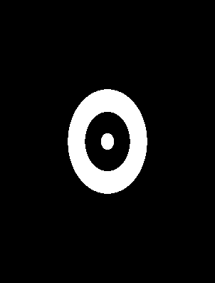 The hardest part of making the filter is the estimation of the concentric circles that we ought to retain. When the filter was already made, we convolve the filter and the FT of the grayscaled fingerprint. The resulting convolution is shown below.
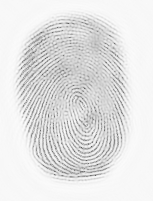 We can observe the removal of the botches and the clearer appearance of the ridges. The ridges are necessary since they make anyone’s fingerprint unique. The botches we encountered are unavoidable since there is an uneven distribution of the ink when we capture our fingerprints. Filtering in the Fourier domain provides us an easy way to process and enhance our images.
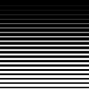
Lunar Landing Scanned Pictures: Line removal
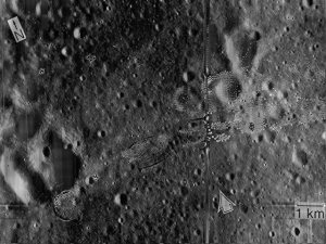
A 1967 lunar picture is shown below. This picture was obtained by the unmanned Lunar Orbiter V spacecraft prior to the Apollo missions to the Moon. The black and white film was automatically developed onboard the spacecraft and
subsequently digitized for transmission to Earth. The regularly spaced vertical lines are the result of combining individually digitized ‘framelets’ to make a composite photograph and the irregularly-shaped bright and dark spots are due to nonuniform film development [3].
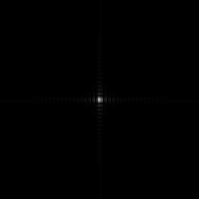
 The lines are the unwanted repetitive patterns for this image. We remove this in the Fourier space. The FT of the grayscaled version of the image is shown below.
 The lines along the x and y axes are the frequencies of the unwanted repetitive line patterns. We need to retain the small circle in the middle as it contains the important information of the picture. Unlike in the case of the fingerprint, we retain the other areas and just completely eliminate the vertical and horizontal lines in the axes. The filter used for the enhancement of the figure is shown below.

The circle in the middle was effectively filtered and the lines in the axes were eliminated. The resulting FT of the convolution of the filter and the FT of the grayscaled image is as follows.
The image on the left side is the product of the filter and the grayscale version of the original image. The right side is the product of the filter applied to the RGB channels of the original image. As we can see for both products, the unwanted repetitive lines are clearly removed using the filter. The method of filtering in the Fourier domain proved to be an effective way of enhancing these images.
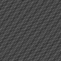
Canvas Weave Modeling and Removal
The last part of the activity directs us to modeling a canvas weave and eventually enhancing a painting by removing the said unwanted part of the image. The image considered is shown below.
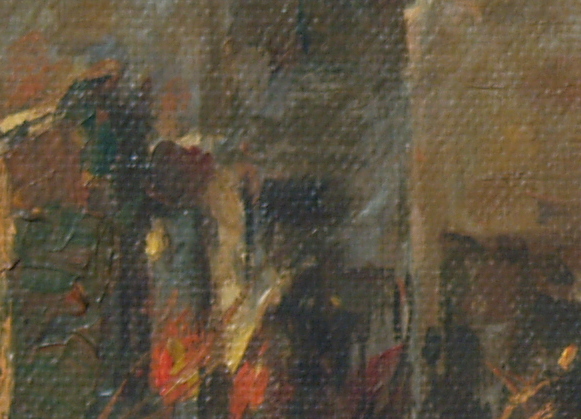
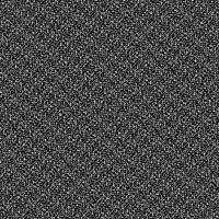
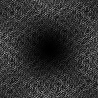
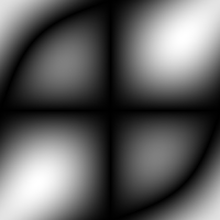
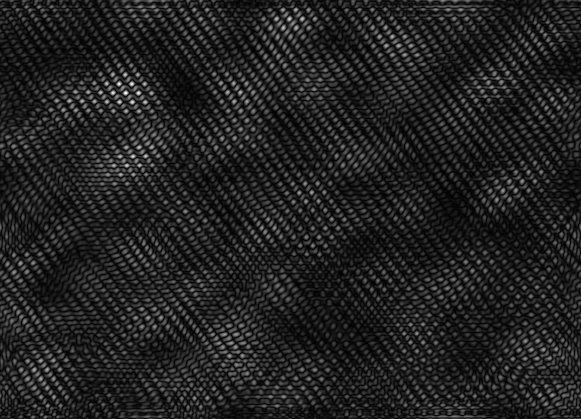
As we can observe, the image of the painting has the obvious patterns of the canvas weave. The pattern is what we aim to remove to enhance the detail of the oil painting. The FT of the grayscale version of this image is given below.
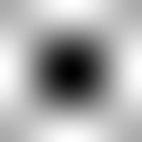
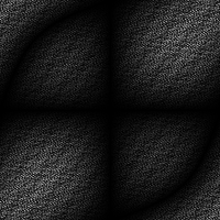
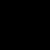
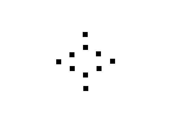
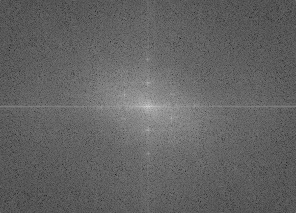 The unwanted repetitive pattern given by the canvas weave is defined by the blots in surrounding the middle area of the FT. These are the patterns we need to remove from the FT image while retaining the entire area, the lines in the axes and the circle in the middle. Using GIMP, I covered these blots using black squares. The filter produced in the process is shown below.
Applying the filter to the FT of the grayscale image of the oil painting, we obtained the FT of the convolution given by the images below.
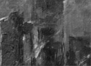
The left side is the product of the filter and the grayscale image of the oil painting. The right image results from the application of the filter to the RGB channels of the original image. For both results, we observe that we have completely removed the canvas weave pattern. The brushstrokes are also improved as observed in the colored result. We completely enhanced the image using the method of filtering in the Fourier domain. If we inverse the filter and convolve it with the FT of the image of the oil painting, we would get the canvas weave pattern. We can therefore conclude that inversing the filter, we could obtain the unwanted repetitive patterns we removed from the images.

The activity was a whole lot of fun. I want to thank Ralph Aguinaldo, Ron Aves, Gio Jubilo, Martin Bartolome and Jaime Olivares for helping me realize some mistakes I made in my Scilab codes. They also provide suggestions most especially on the last 3 sets of activities of enhancing images by filtering in the Fourier domain. Honestly, I overthinked a lot of these activities. The activity made me realize that some things even how complicated it may seem, is just simple as saying 1-2-3. I feel like I would have completed the activity much earlier if I did not give too much time in finding ways to produce an image of my fingerprint.
Overall, the activity was both stressful yet fulfilling. Since I completed every part of the activity and produce very good results, I would give myself a 10 for this activity. I believe, I was also able to place good insights about the theories behind the results obtained for this activity. I also know that I do not deserve extra points due to the punctuality of my blog. But still, regardless of points, I feel really cool producing my results. And nobody would stop me from feeling this way.

References:
- A6 – Properties and Applications of the 2D Fourier Transform, Dr. Maricor Soriano, Applied Physics 186 Manual
- Anamorphic, http://www.merriam-webster.com/dictionary/anamorphic
- Lunar Picture from Lunar Orbiter V spacecraft, http://www.lpi.usra.edu/lunar/missions/apollo/apollo_11/images/
